An R Companion to Chapter 1 of Hosmer, Lemeshow and Sturdivant’s Applied Linear Regression
This post is an R illustration of the first chapter of Hosmer, David W., Stanley Lemeshow, and Rodney X. Sturdivant. Applied logistic regression. Hoboken, New Jersey: Wiley, 2013, the standard text (HLS). Chapter 1 introduces the logistic regression model, how to fit one, test the significance of its coefficients and calculate its confidence intervals. It also discusses other estimation methods, and introduces the datasets used in the book’s examples and exercises. There are three exercises. The chapter is 33 pages long.
Source data
The datasets are available as zip files at the publisher’s data website with 9780470582473 as the search term. The unzipped .txt files are tab delimited. It is assumed that readers are familiar with importing such datasets into R workspaces using tools such as readr::read_tsv(). Note that it will be convenient to bulk download and unzip the files into subdirectories of your workspace, due to the organization of the data website.
The example code assumes that a directory named data is a direct subdirectory of your working directory and that each dataset is in a sudirectory of data, as follows:
data
├── APS
    │   ├── APS_Code_Sheet.pdf
    │   └── APS.txt
    ├── BURN
    │   ├── BURN1000.txt
    │   ├── BURN13M.txt
    │   ├── BURN_Code_Sheet.pdf
    │   ├── BURN_EVAL_1.txt
    │   └── BURN_EVAL_2.txt
    ├── CHDAGE
    │   ├── CHDAGE_Code_Sheet.pdf
    │   └── CHDAGE.txt
    ├── GLOW
    │   ├── GLOW11M.txt
    │   ├── GLOW500.txt
    │   ├── GLOW_BONEMED.txt
    │   ├── GLOW_Code_Sheet.pdf
    │   ├── GLOW_MIS_Comp_Data.txt
    │   ├── GLOW_MIS_WMissing_Data.txt
    │   └── GLOW_RAND.txt
    ├── ICU
    │   ├── ICU_Data_Code_Sheet.pdf
    │   └── ICU.txt
    ├── LOWBWT
    │   ├── LOWBWT_Code_Sheet.pdf
    │   └── LOWBWT.txt
    ├── MYOPIA
    │   ├── MYOPIA_Code_Sheet.pdf
    │   └── MYOPIA.txt
    ├── NHANES
    │   ├── NHANES_Code_Sheet.pdf
    │   └── NHANES.txt
    ├── POLYPHARM
    │   ├── POLYPHARM_Code_Sheet.pdf
    │   └── POLYPHARM.txt
    ├── Scale Example
    │   ├── Scale.Example.code.sheet.docx
    │   ├── Scale.Example.code.sheet.pdf
    │   ├── Scale_Example.out
    │   ├── Scale_Example.tab.txt
    │   ├── Scale_Example.txt
    │   └── Scale_Example.xlsx
Code for text tables and figures
Section 1.1
Table 1.1
Table 1.1 displays the 100 records of the CHDAGE dataset with a constructed age group column, AGEGRP.
chdage <- readr::read_tsv("data/CHDAGE/CHDAGE.txt")

# Classify ages into 5- or 10-year cohorts

df1.1 <-  chdage %>% mutate(cohort = ifelse(AGE < 30,1, 0))
df1.1 <- df1.1 %>% mutate(cohort = ifelse(AGE >= 30 & AGE <= 34,2, cohort))
df1.1 <- df1.1 %>% mutate(cohort = ifelse(AGE >= 30 & AGE <= 34,2, cohort))
df1.1 <- df1.1 %>% mutate(cohort = ifelse(AGE >= 35 & AGE <= 39,3, cohort))
df1.1 <- df1.1 %>% mutate(cohort = ifelse(AGE >= 40 & AGE <= 44,4, cohort))
df1.1 <- df1.1 %>% mutate(cohort = ifelse(AGE >= 45 & AGE <= 49,5, cohort))
df1.1 <- df1.1 %>% mutate(cohort = ifelse(AGE >= 50 & AGE <= 54,6, cohort))
df1.1 <- df1.1 %>% mutate(cohort = ifelse(AGE >= 55 & AGE <= 59,7, cohort))
df1.1 <- df1.1 %>% mutate(cohort = ifelse(AGE >= 60 & AGE <= 90,8, cohort))

# use medians of cohort endpoints for plotting
    # medians obtained by hand using md function
    #
    df1.2 <- df1.1 %>% mutate(plotpoint = ifelse(cohort == 1,24.5, 0))
    df1.2 <- df1.2 %>% mutate(plotpoint = ifelse(cohort == 2,32, plotpoint))
    df1.2 <- df1.2 %>% mutate(plotpoint = ifelse(cohort == 3,37, plotpoint))
    df1.2 <- df1.2 %>% mutate(plotpoint = ifelse(cohort == 4,42, plotpoint))
    df1.2 <- df1.2 %>% mutate(plotpoint = ifelse(cohort == 5,47, plotpoint))
    df1.2 <- df1.2 %>% mutate(plotpoint = ifelse(cohort == 6,52, plotpoint))
    df1.2 <- df1.2 %>% mutate(plotpoint = ifelse(cohort == 7,57, plotpoint))
    df1.2 <- df1.2 %>% mutate(plotpoint = ifelse(cohort == 8,65, plotpoint))

    # Create a text column for cohort lables

    df1.2 <- df1.2 %>% mutate(AGEGRP = ifelse(cohort == 1,"20-29", 0))
    df1.2 <- df1.2 %>% mutate(AGEGRP = ifelse(cohort == 2,"30-34", AGEGRP))
    df1.2 <- df1.2 %>% mutate(AGEGRP = ifelse(cohort == 3,"35-39", AGEGRP))
    df1.2 <- df1.2 %>% mutate(AGEGRP = ifelse(cohort == 4,"40-44", AGEGRP))
    df1.2 <- df1.2 %>% mutate(AGEGRP = ifelse(cohort == 5,"45-49", AGEGRP))
    df1.2 <- df1.2 %>% mutate(AGEGRP = ifelse(cohort == 6,"50-54", AGEGRP))
    df1.2 <- df1.2 %>% mutate(AGEGRP = ifelse(cohort == 7,"55-59", AGEGRP))
    df1.2 <- df1.2 %>% mutate(AGEGRP = ifelse(cohort == 8,"60-70", AGEGRP))

    # split CHD column

    df1.2 <- df1.2 %>% mutate(absent  = ifelse(CHD == 0,1,0))
df1.2 <- df1.2 %>% mutate(present = ifelse(CHD == 1,1,0))| ID | AGE | AGEGRP | CHD |
|---|---|---|---|
| 1 | 20 | 20-29 | 0 |
| 2 | 23 | 20-29 | 0 |
| 3 | 24 | 20-29 | 0 |
| 5 | 25 | 20-29 | 1 |
| 4 | 25 | 20-29 | 0 |
| 7 | 26 | 20-29 | 0 |
| 6 | 26 | 20-29 | 0 |
| 9 | 28 | 20-29 | 0 |
| 8 | 28 | 20-29 | 0 |
| 10 | 29 | 20-29 | 0 |
| 11 | 30 | 30-34 | 0 |
| 13 | 30 | 30-34 | 0 |
| 16 | 30 | 30-34 | 1 |
| 14 | 30 | 30-34 | 0 |
| 15 | 30 | 30-34 | 0 |
| 12 | 30 | 30-34 | 0 |
| 18 | 32 | 30-34 | 0 |
| 17 | 32 | 30-34 | 0 |
| 19 | 33 | 30-34 | 0 |
| 20 | 33 | 30-34 | 0 |
| 24 | 34 | 30-34 | 0 |
| 22 | 34 | 30-34 | 0 |
| 23 | 34 | 30-34 | 1 |
| 21 | 34 | 30-34 | 0 |
| 25 | 34 | 30-34 | 0 |
| 27 | 35 | 35-39 | 0 |
| 26 | 35 | 35-39 | 0 |
| 29 | 36 | 35-39 | 1 |
| 28 | 36 | 35-39 | 0 |
| 30 | 36 | 35-39 | 0 |
| 32 | 37 | 35-39 | 1 |
| 33 | 37 | 35-39 | 0 |
| 31 | 37 | 35-39 | 0 |
| 35 | 38 | 35-39 | 0 |
| 34 | 38 | 35-39 | 0 |
| 37 | 39 | 35-39 | 1 |
| 36 | 39 | 35-39 | 0 |
| 39 | 40 | 40-44 | 1 |
| 38 | 40 | 40-44 | 0 |
| 41 | 41 | 40-44 | 0 |
| 40 | 41 | 40-44 | 0 |
| 43 | 42 | 40-44 | 0 |
| 44 | 42 | 40-44 | 0 |
| 45 | 42 | 40-44 | 1 |
| 42 | 42 | 40-44 | 0 |
| 46 | 43 | 40-44 | 0 |
| 47 | 43 | 40-44 | 0 |
| 48 | 43 | 40-44 | 1 |
| 50 | 44 | 40-44 | 0 |
| 51 | 44 | 40-44 | 1 |
| 52 | 44 | 40-44 | 1 |
| 49 | 44 | 40-44 | 0 |
| 53 | 45 | 45-49 | 0 |
| 54 | 45 | 45-49 | 1 |
| 55 | 46 | 45-49 | 0 |
| 56 | 46 | 45-49 | 1 |
| 59 | 47 | 45-49 | 1 |
| 58 | 47 | 45-49 | 0 |
| 57 | 47 | 45-49 | 0 |
| 60 | 48 | 45-49 | 0 |
| 62 | 48 | 45-49 | 1 |
| 61 | 48 | 45-49 | 1 |
| 65 | 49 | 45-49 | 1 |
| 63 | 49 | 45-49 | 0 |
| 64 | 49 | 45-49 | 0 |
| 67 | 50 | 50-54 | 1 |
| 66 | 50 | 50-54 | 0 |
| 68 | 51 | 50-54 | 0 |
| 70 | 52 | 50-54 | 1 |
| 69 | 52 | 50-54 | 0 |
| 71 | 53 | 50-54 | 1 |
| 72 | 53 | 50-54 | 1 |
| 73 | 54 | 50-54 | 1 |
| 75 | 55 | 55-59 | 1 |
| 76 | 55 | 55-59 | 1 |
| 74 | 55 | 55-59 | 0 |
| 78 | 56 | 55-59 | 1 |
| 77 | 56 | 55-59 | 1 |
| 79 | 56 | 55-59 | 1 |
| 82 | 57 | 55-59 | 1 |
| 84 | 57 | 55-59 | 1 |
| 80 | 57 | 55-59 | 0 |
| 85 | 57 | 55-59 | 1 |
| 81 | 57 | 55-59 | 0 |
| 83 | 57 | 55-59 | 1 |
| 86 | 58 | 55-59 | 0 |
| 87 | 58 | 55-59 | 1 |
| 88 | 58 | 55-59 | 1 |
| 90 | 59 | 55-59 | 1 |
| 89 | 59 | 55-59 | 1 |
| 91 | 60 | 60-70 | 0 |
| 92 | 60 | 60-70 | 1 |
| 93 | 61 | 60-70 | 1 |
| 94 | 62 | 60-70 | 1 |
| 95 | 62 | 60-70 | 1 |
| 96 | 63 | 60-70 | 1 |
| 98 | 64 | 60-70 | 1 |
| 97 | 64 | 60-70 | 0 |
| 99 | 65 | 60-70 | 1 |
| 100 | 69 | 60-70 | 1 |
Figure 1.1
Figure 1.1 is a scatterplot of coronary heart disease against age in the CHDAGE dataset.
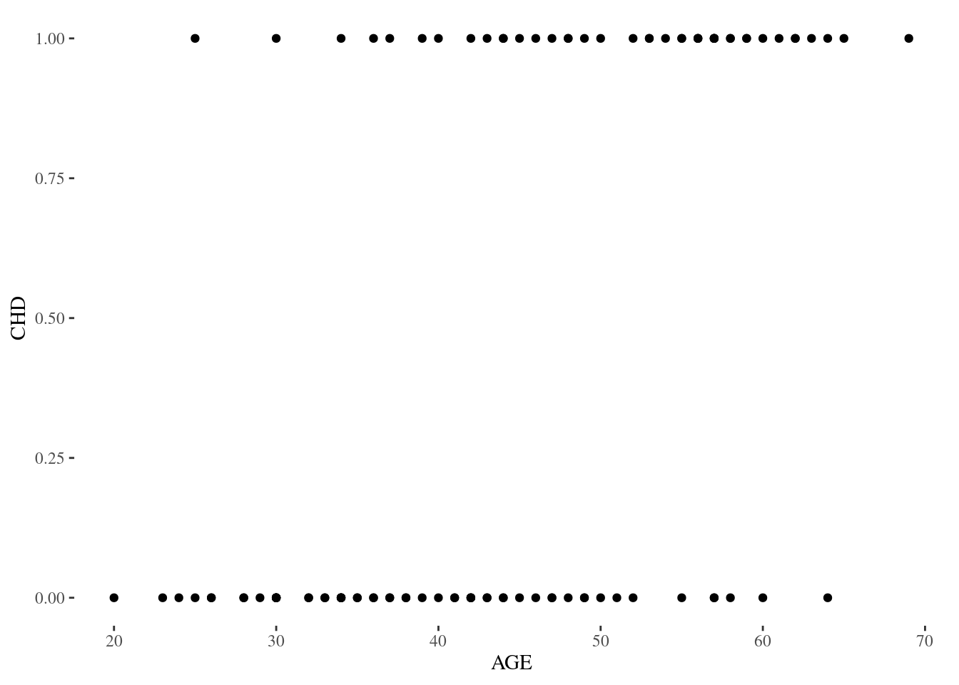
produced with
p1.1 <- ggplot(data = chdage, aes(x = AGE, y = CHD)) + geom_point() + theme_tufte()Commentary: It’s also instructive to look at the results of
fit1.1 <- lm(CHD ~ AGE, data = chdage)in a plot produced with
par(mfrow=c(2,2))
plot(fit1.1)
compared to a plot from the mtcars dataset of mpg ~ hp

Table 1.2
Table 1.2 shows the frequency and means of CHD (coronary heart disease)in the CHDAGE dataset by age cohort, produced as follows:
    # Create table with plotting information
    #
    means_tab <- df1.2 %>% group_by(AGEGRP) %>%
      summarize(n = n(), Absent = sum(absent),
      Present = sum(present), Mean = mean(CHD),
      plotpoint = mean(plotpoint)) %>% ungroup()

Table 1.3
Table 1.3 presents the result of a logistic model of the CHD against age in the CHDAGE dataset. The equivalent is produced in R by the glm function in {stats} as follows:
chdfit <- glm(CHD ~ AGE, data = chdage, family = binomial(link =
"logit"))
summary(chdfit)
##
## Call:
## glm(formula = CHD ~ AGE, family = binomial(link = "logit"), data = chdage)
##
## Deviance Residuals:
## Min 1Q Median 3Q Max
## -1.9718 -0.8456 -0.4576 0.8253 2.2859
##
## Coefficients:
## Estimate Std. Error z value Pr(>|z|)
## (Intercept) -5.30945 1.13365 -4.683 2.82e-06 ***
## AGE 0.11092 0.02406 4.610 4.02e-06 ***
## ---
## Signif. codes: 0 '***' 0.001 '**' 0.01 '*' 0.05 '.' 0.1 ' ' 1
##
## (Dispersion parameter for binomial family taken to be 1)
##
## Null deviance: 136.66 on 99 degrees of freedom
## Residual deviance: 107.35 on 98 degrees of freedom
## AIC: 111.35
##
## Number of Fisher Scoring iterations: 4Note that the standard summary for glm does not produce log likelihood, and it is necessary to call logLik separately.
logLik(chdfit)## 'log Lik.' -53.67655 (df=2)The text identifies three methods of calculating confidence intervals for the model fit of the coefficients: the Wald-based confidence interval estimator and the likelihood ratio test on pages 18-19, and the “Score test” on page 14.1 I refer to these as waldscore, vmscore2 and raoscore.
Given a fitted model, two are easy to calculate:
library(MASS)
waldscore <- confint.default(chdfit)
waldscore
## 2.5 % 97.5 %
## (Intercept) -7.53137370 -3.0875331
## AGE 0.06376477 0.1580775vmscore <- confint(chdfit)## Waiting for profiling to be done...vmscore## 2.5 % 97.5 %
## (Intercept) -7.72587162 -3.2461547
## AGE 0.06693158 0.1620067The third depends on the profileModel package
library(profileModel)
raoscore <- profConfint(profileModel(chdfit, quantile=qchisq(0.95, 1), objective = "RaoScoreStatistic", X = model.matrix(chdfit)))
## Preliminary iteration .. Done
##
## Profiling for parameter (Intercept) ... Done
## Profiling for parameter AGE ... Doneattr(raoscore, "dimnames")[2][[1]] <- c("2.5 %","97.5 %")
raoscore <- raoscore[,1:2]
raoscore## 2.5 % 97.5 %
## (Intercept) -7.50801115 -3.1218722
## AGE 0.06448682 0.1575531Table 1.4
Table 1.4., the covariance matrix of the estimated coefficients in Table 1.3, is produced by in equivalent form by
vcov(chdfit)## (Intercept) AGE
## (Intercept) 1.28517059 -0.0266769747
## AGE -0.02667697 0.0005788748Figure 1.3
Figure 1.3 plots the profile log likelihood for the AGE variable in the CDHAGE dataset. See the discussion on page 19 of HLS. It can be produced with the following code
library(dplyr)
library(purrr)
library(ggplot2)


get_profile_glm <- function(aglm){
  prof <- MASS:::profile.glm(aglm, del = .05, maxsteps = 52)
  disp <- attr(prof,"summary")$dispersion
  purrr::imap_dfr(prof, .f = ~data.frame(par = .y,
                  deviance=.x$z^2*disp+aglm$deviance,
                  values = as.data.frame(.x$par.vals)[[.y]], stringsAsFactors = FALSE))
}

chdage <- readr::read_tsv("data/CHDAGE/CHDAGE.txt")
## Parsed with column specification:
## cols(
## ID = col_double(),
## AGE = col_double(),
## CHD = col_double()
## )chdfit <- glm(CHD ~ AGE, data = chdage, family = binomial(link = "logit"))
pll <- get_profile_glm(chdfit) %>% filter(par == "AGE") %>% mutate(beta = values) %>% mutate(pll = deviance * -0.5) %>% dplyr::select(-c(par,values, deviance))
asymmetry <- function(x) {
ci <- confint(x, level = 0.95)
ci_lower <- ci[2,1]
ci_upper <- ci[2,2]
coeff <- x$coefficients[2]
round(100 * ((ci_upper - coeff) - (coeff - ci_lower))/(ci_upper - ci_lower), 2)
}
asym <- asymmetry(chdfit)## Waiting for profiling to be done...ggplot(data = pll, aes(x = beta, y = pll)) +
geom_line() +
scale_x_continuous(breaks = c(0.06, 0.08, 0.10, 0.12, 0.14, 0.16)) +
scale_y_continuous(breaks = c(-57, -56, -55, -54)) +
xlab("Coefficient for age") +
ylab("Profile log-likelihood function") +
geom_vline(xintercept = confint(chdfit)[2,1]) +
geom_vline(xintercept = confint(chdfit)[2,2]) +
geom_hline(yintercept = (logLik(chdfit) - (qchisq(0.95, df = 1)/2))) +
theme_classic() +
ggtitle(paste("Asymmetry =", scales::percent(asym/100, accuracy = 0.1))) + theme(plot.title = element_text(hjust = 0.5))## Waiting for profiling to be done...## Waiting for profiling to be done...
For a brief discussion of development of the get_profile_glm function, see this stackoverflow post. Note that the arguments to
prof <- MASS:::profile.glm(chdfit, del = .05, maxsteps = 52)were hand selected specifically for this example and will likely require adjustment for different data.
Commentary
Chapter 1 is foundational. Understanding it adequately is key to further progress. Parsing the equations is part of the task. It is helpful to write them out in an equation formatter, such as \(\LaTeX\), which is built into RStudio.
Equation 1.1
To produce
\[\pi(x) = \frac{e^{\beta{_0}+\beta{_1}x}}{1 + e^{\beta{_0}+\beta{_1}x}}\]
and
\[g(x) = ln\Bigl[\frac{\pi(x)}{1 - \pi(x)}\Big] = \beta_0 +\beta_1x\]
write
$$pi(x) = \frac{e^{\beta{_0}+\beta{_1}x}}{1 + e^{\beta{_0}+\beta{_1}$$
and
$$g(x) = ln\Bigl[\frac{\pi(x)6}{1 - \pi(x)}\Big] = \beta_0 +\beta_1x$$
Equation 1.2
\[\pi(x_i)^{y_i}[1 - \pi(x_i)]^{1-y_i}\]
Equation 1.3
\[l\beta = \prod_{i = 1}^n\pi(x)^{y_i}[1 - \pi(x)]^{1-y_i}, n = 200\]
Equation 1.4
\[L(\beta) = ln[l(\beta)] = \sum_{i = 1}^{n}[y_i, ln[\pi(x_i)] + (1 - y_i)ln[1 -\pi(x-i)])\]