## Please note: Alaska and Hawaii are being shifted and are not to scale.Color, Design and Communication
Graphic design standards, especially for color, are an official Good Thing. Branding, visual cueing, consistency. Map colors are hard, especially when dealing with continuous data.
An example of continuous data
The U.S. Bureau of Economic Analysis publishes quarterly statistics on gross domestic product by state.1. For the second quarter 2018, it provided the following.
| NAME | GDP | geometry |
|---|---|---|
| Arizona | 322,995 | MULTIPOLYGON (((-1111066 -8… |
| Arkansas | 123,605 | MULTIPOLYGON (((557903.1 -1… |
| California | 2,791,626 | MULTIPOLYGON (((-1853480 -9… |
| Colorado | 343,316 | MULTIPOLYGON (((-613452.9 -… |
| Connecticut | 264,949 | MULTIPOLYGON (((2226838 519… |
| Georgia | 557,294 | MULTIPOLYGON (((1379893 -98… |
| Illinois | 820,408 | MULTIPOLYGON (((868942.5 -2… |
| Indiana | 348,366 | MULTIPOLYGON (((1279733 -39… |
| Louisiana | 236,514 | MULTIPOLYGON (((1080885 -16… |
| Minnesota | 351,868 | MULTIPOLYGON (((594664.5 21… |
| Mississippi | 109,181 | MULTIPOLYGON (((1052956 -15… |
| Montana | 47,040 | MULTIPOLYGON (((-864991.3 5… |
| New Mexico | 93,323 | MULTIPOLYGON (((-568680.6 -… |
| North Dakota | 51,972 | MULTIPOLYGON (((-39585.46 1… |
| Oklahoma | 187,043 | MULTIPOLYGON (((-34.95064 -… |
| Pennsylvania | 746,635 | MULTIPOLYGON (((1734901 -36… |
| Tennessee | 345,710 | MULTIPOLYGON (((1467705 -78… |
| Virginia | 507,407 | MULTIPOLYGON (((2133159 -45… |
| Delaware | 71,164 | MULTIPOLYGON (((2058738 -29… |
| West Virginia | 72,288 | MULTIPOLYGON (((1827955 -42… |
| Wisconsin | 319,280 | MULTIPOLYGON (((721464.2 26… |
| Wyoming | 37,644 | MULTIPOLYGON (((-324546.2 -… |
| Alabama | 210,298 | MULTIPOLYGON (((1145349 -15… |
| Florida | 971,078 | MULTIPOLYGON (((1994020 -19… |
| Idaho | 72,065 | MULTIPOLYGON (((-873311.5 1… |
| Kansas | 159,167 | MULTIPOLYGON (((40850.31 -8… |
| Maryland | 396,750 | MULTIPOLYGON (((2063382 -46… |
| New Jersey | 597,752 | MULTIPOLYGON (((2096848 -22… |
| North Carolina | 534,880 | MULTIPOLYGON (((2173840 -77… |
| South Carolina | 221,061 | MULTIPOLYGON (((1607185 -91… |
| Washington | 518,701 | MULTIPOLYGON (((-1642369 55… |
| Vermont | 32,490 | MULTIPOLYGON (((2197053 124… |
| Utah | 163,887 | MULTIPOLYGON (((-909692.9 -… |
| Iowa | 183,496 | MULTIPOLYGON (((717165 -185… |
| Kentucky | 199,833 | MULTIPOLYGON (((934668.1 -8… |
| Maine | 61,230 | MULTIPOLYGON (((2391419 325… |
| Massachusetts | 537,860 | MULTIPOLYGON (((2364278 491… |
| Michigan | 503,384 | MULTIPOLYGON (((1112263 184… |
| Missouri | 303,577 | MULTIPOLYGON (((936191 -904… |
| Nebraska | 118,536 | MULTIPOLYGON (((-336456.4 -… |
| Nevada | 155,890 | MULTIPOLYGON (((-1188405 -4… |
| New Hampshire | 80,427 | MULTIPOLYGON (((2305592 212… |
| New York | 1,583,899 | MULTIPOLYGON (((2160781 -11… |
| Ohio | 641,630 | MULTIPOLYGON (((1425651 -22… |
| Oregon | 224,764 | MULTIPOLYGON (((-1676653 30… |
| Rhode Island | 59,201 | MULTIPOLYGON (((2325633 198… |
| South Dakota | 49,706 | MULTIPOLYGON (((-325003.8 -… |
| Texas | 1,640,409 | MULTIPOLYGON (((314225.2 -1… |
| Alaska | 51,214 | MULTIPOLYGON (((-1434617 -2… |
| Hawaii | 88,593 | MULTIPOLYGON (((-231495.6 -… |
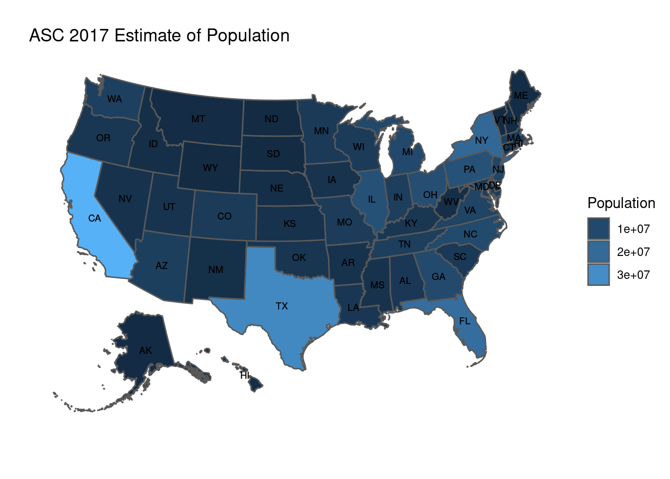
The two obvious things from the chart are that the numbers differ and that in general the larger states in population are also the larger states in GDP. Whenever making maps of continuous data, they will almost always turn out like this, unless there are marked regional differences and you take the default option.
Here is the GDP data, also with the default option.
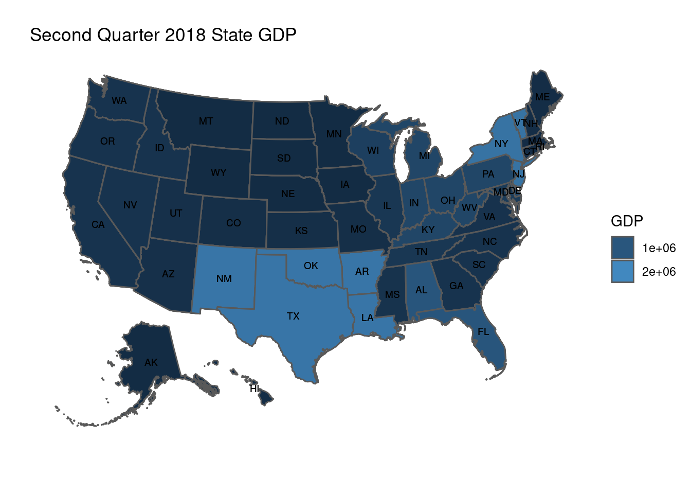
Three Problems: One Major, One Important and One Nuisance
- Major: The GDP map doesn’t tell you anything you could not have guessed from the population map
- You can see subtle differences in shade, but there are too many, and a small portion of the population is blue colorblind.
- Nuisance: Can’t see the state names against the dark background
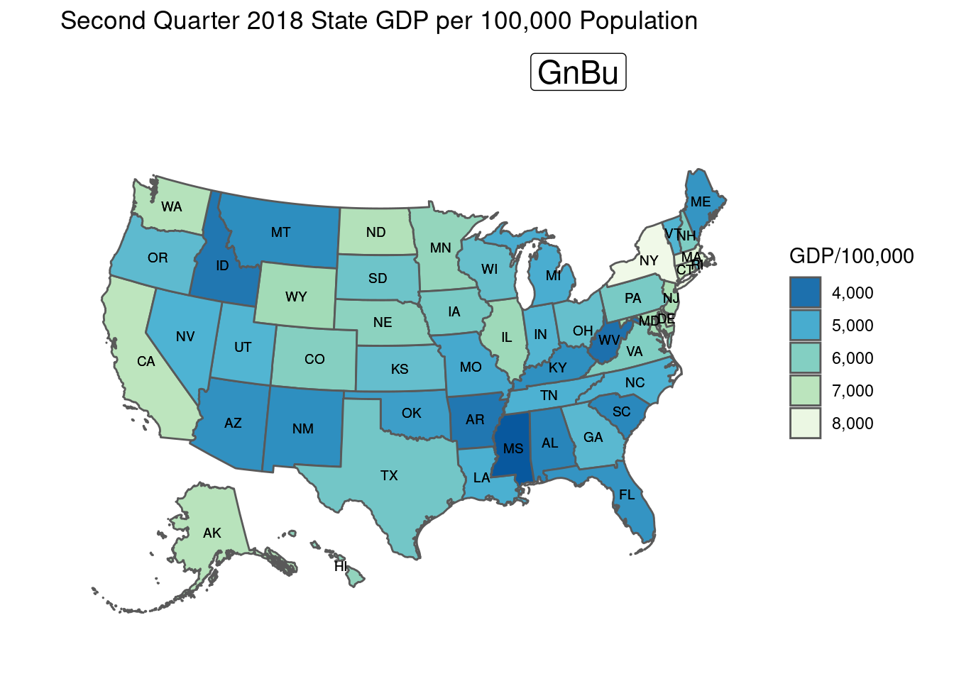
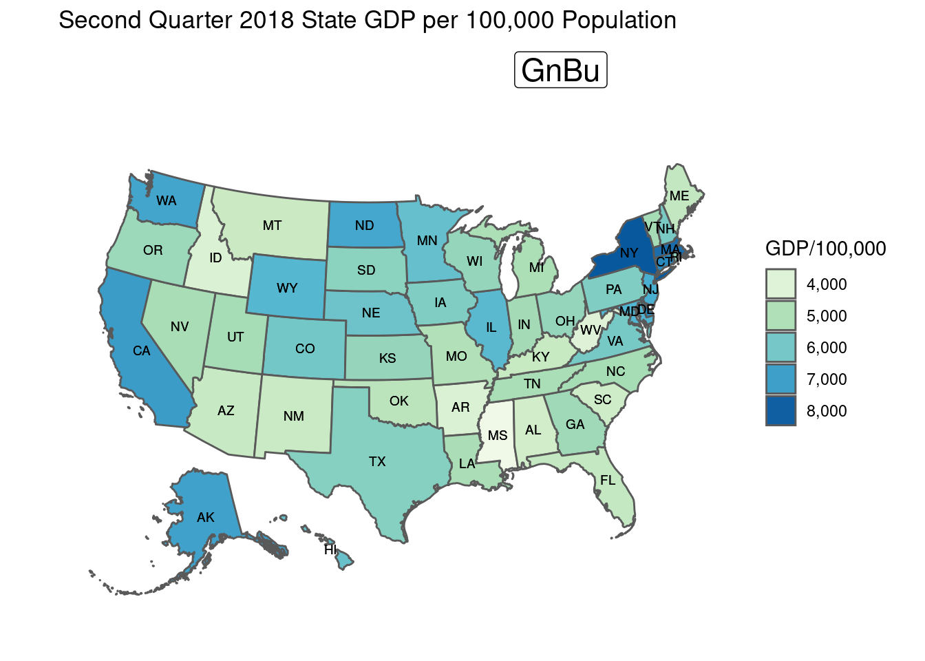
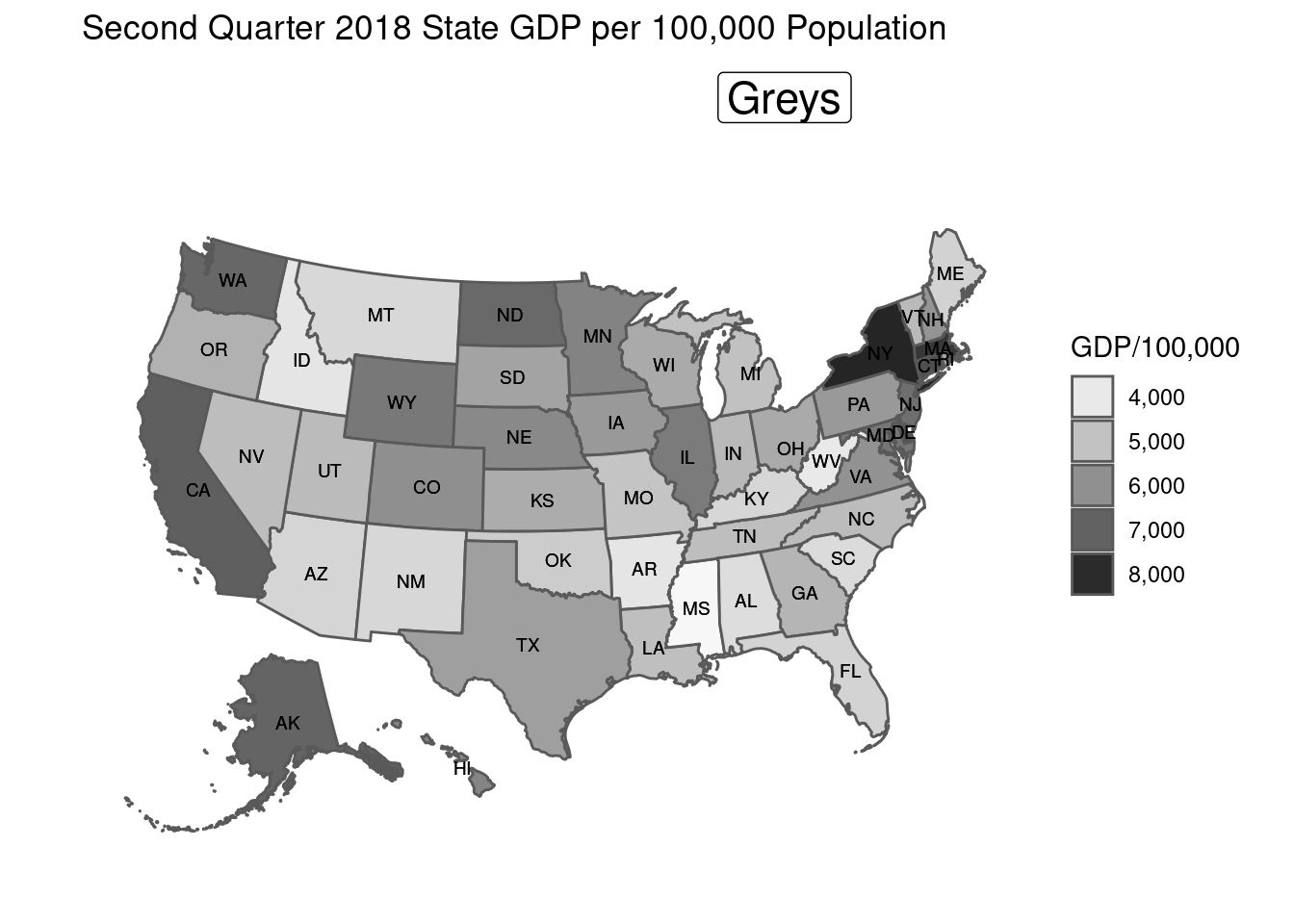
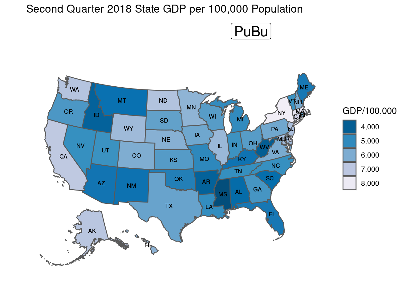
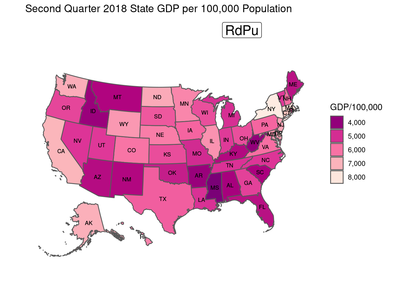
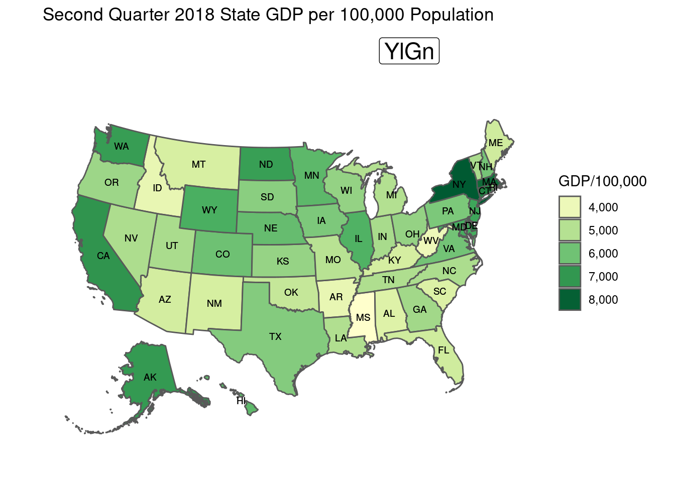
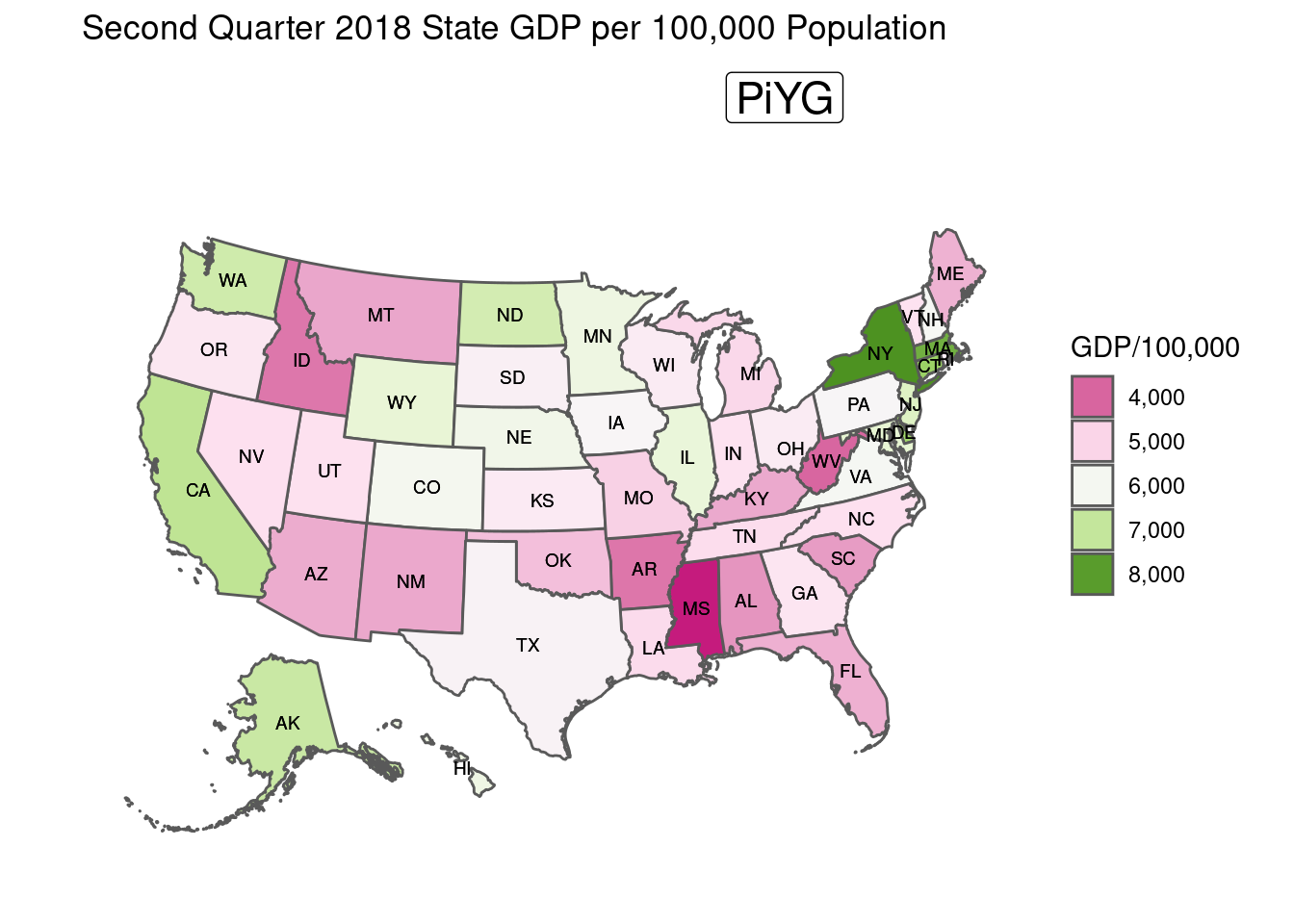
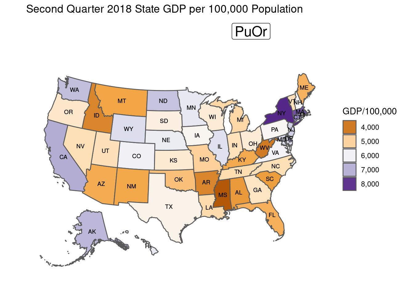
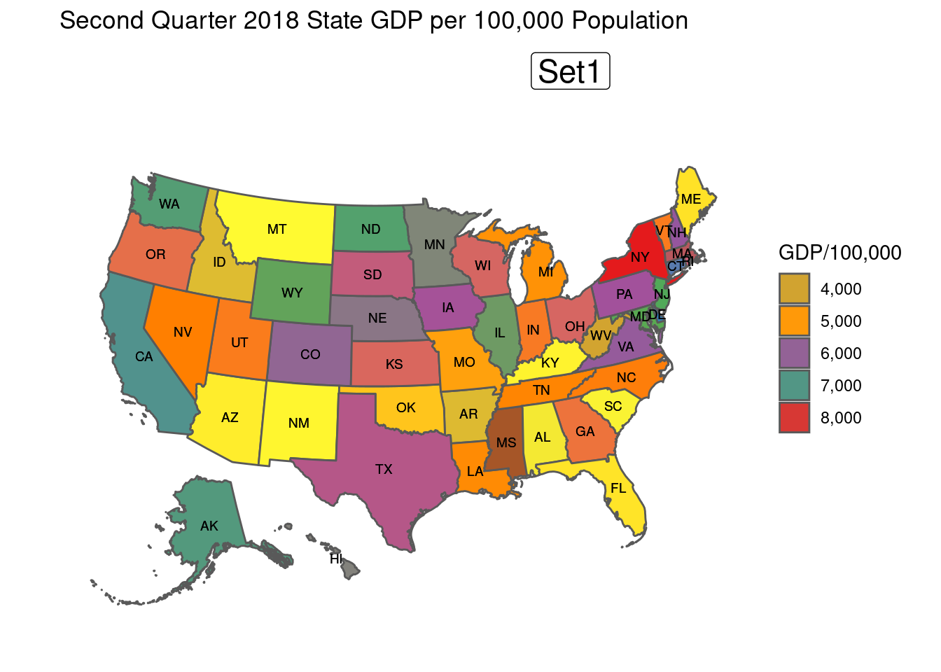
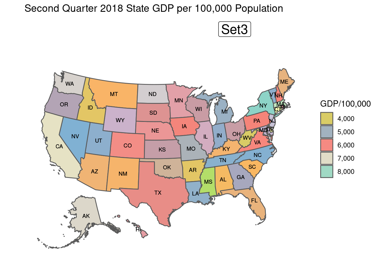
The Major Problem: Counts Need Transformation
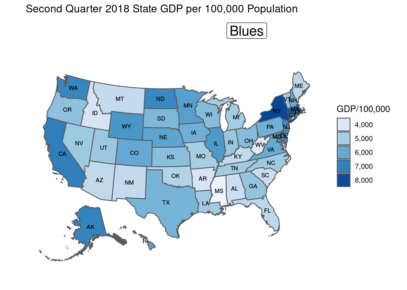
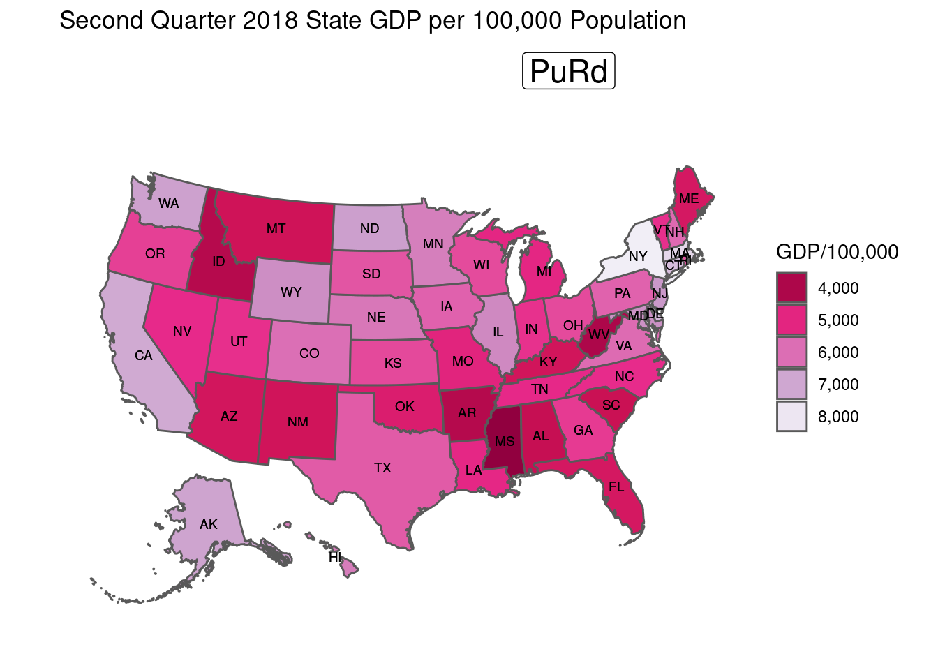
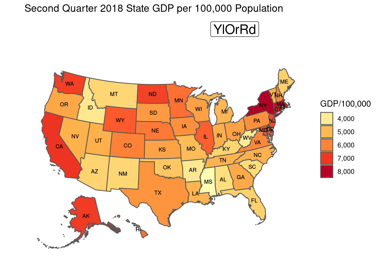
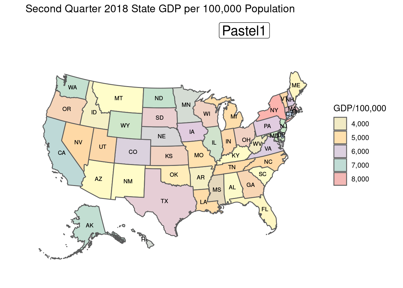
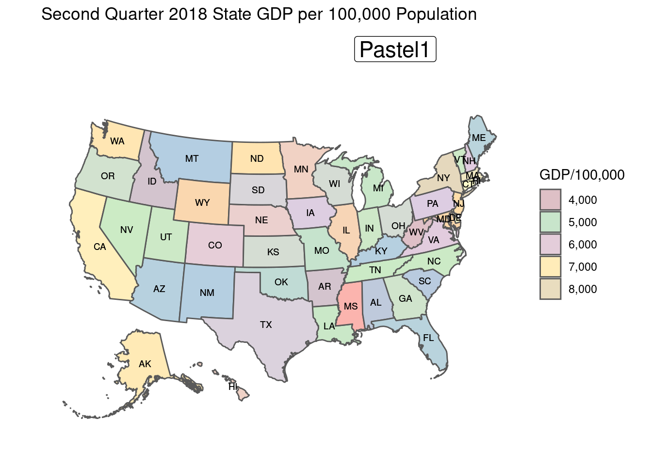
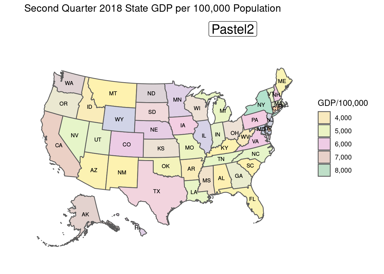
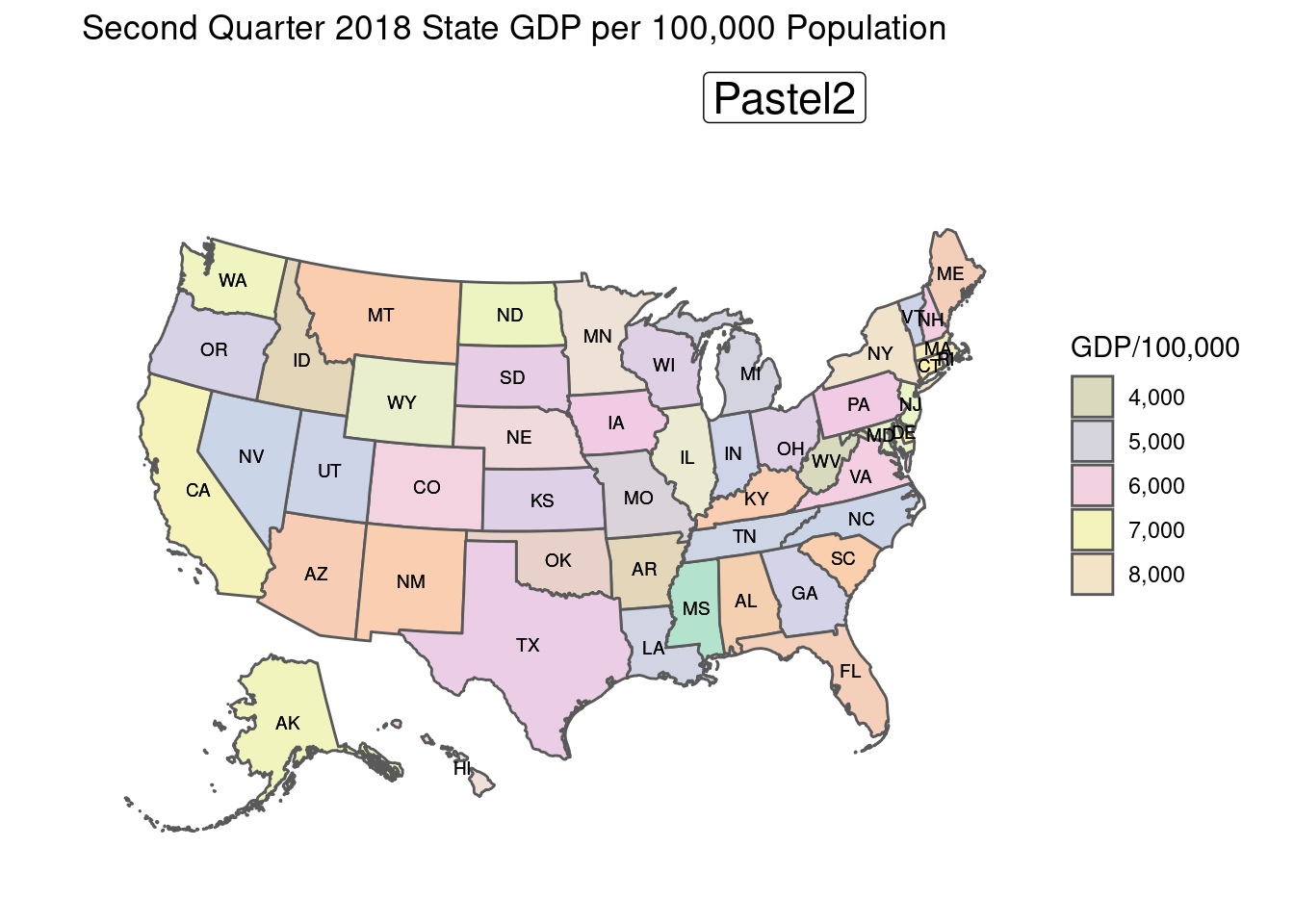
If we are looking for more interesting differences among states, we should put them on a common footing, so that population size alone doesn’t dominate the effects. For disease, as an example, cases per hundred thousand is commonly used. Here’s what the GDP data looks like on that basis.
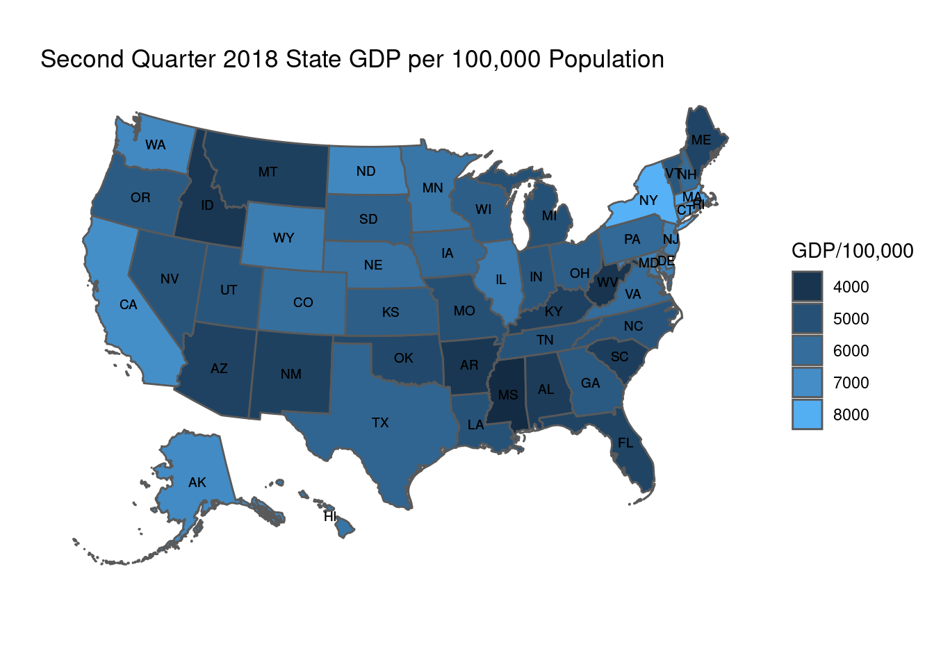
The Important Problem
The default continuous blue scale, even with transformed data, still requires squinting to distinguish different values.
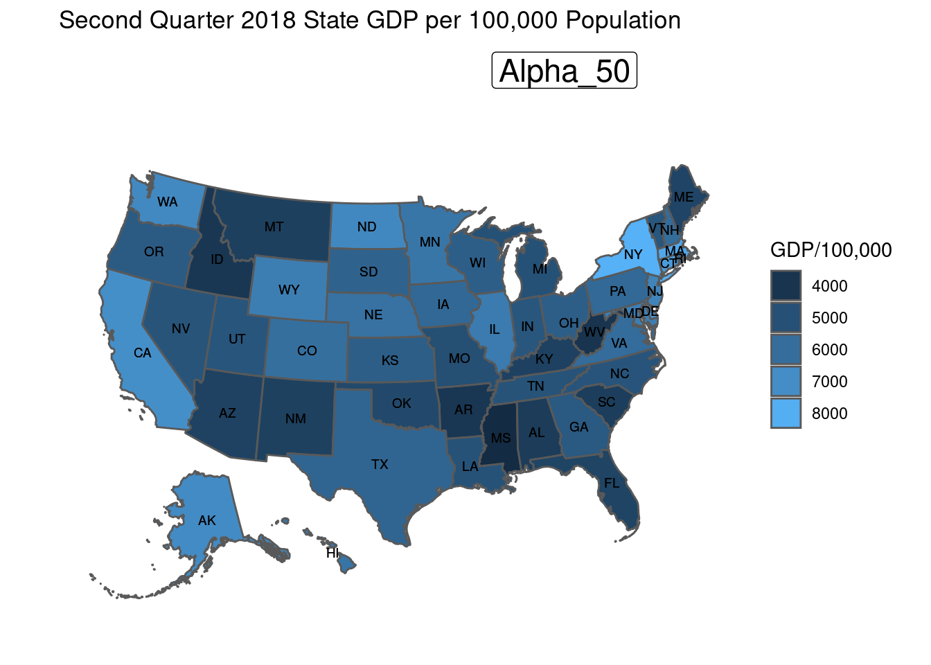
Alpha adjustment
We can tinker with that by applying an alpha (density) filter.

The signature for scale_alpha_continuous is
scale_alpha_continuous(…, range = c(0.1, 1))
The range can be narrowed

scale_alpha_continuous(range = c(0.1, 0.75))
or even further lightened
scale_alpha_continuous(range = c(0.1, 0.50))
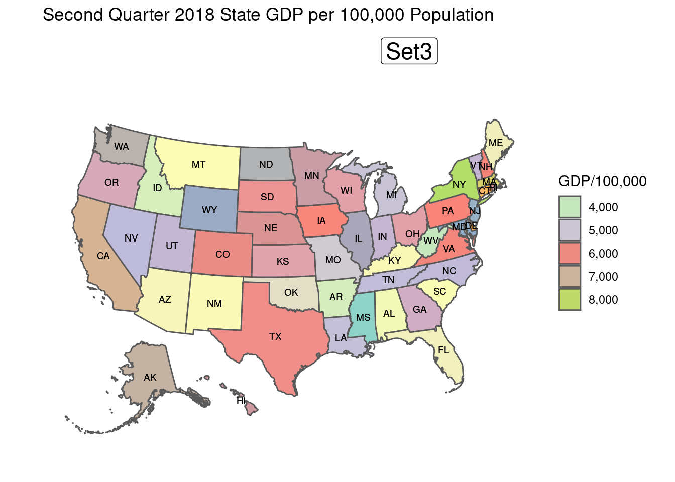
Beyond Blue Palette Solutions
Viridis palette
Five bright (some might say garish) scales are available.
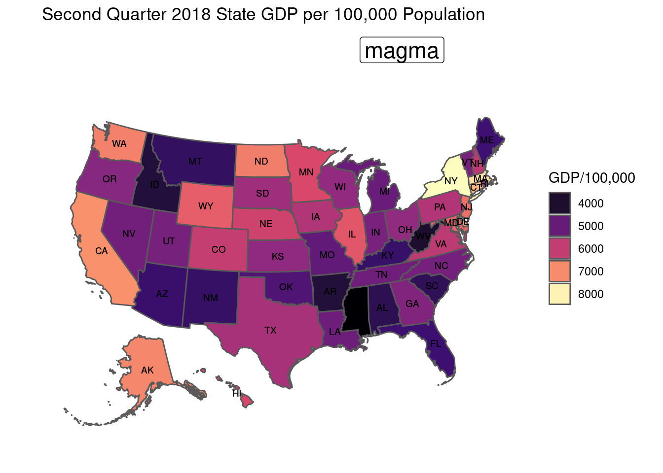
scale_fill_viridis_c(option="magma")
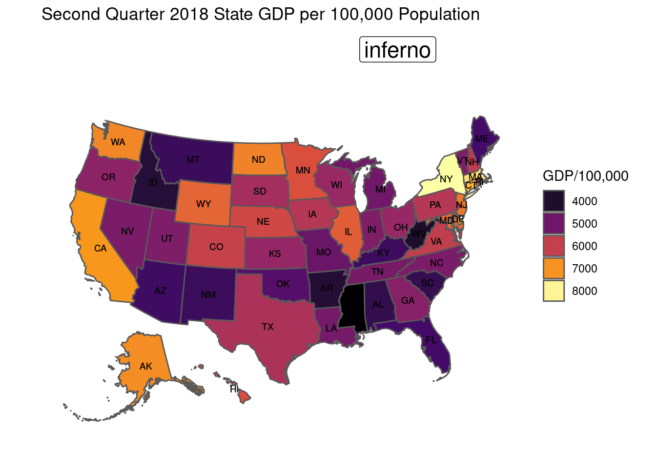
scale_fill_viridis_c(option="inferno")

scale_fill_viridis_c(option="plasma")
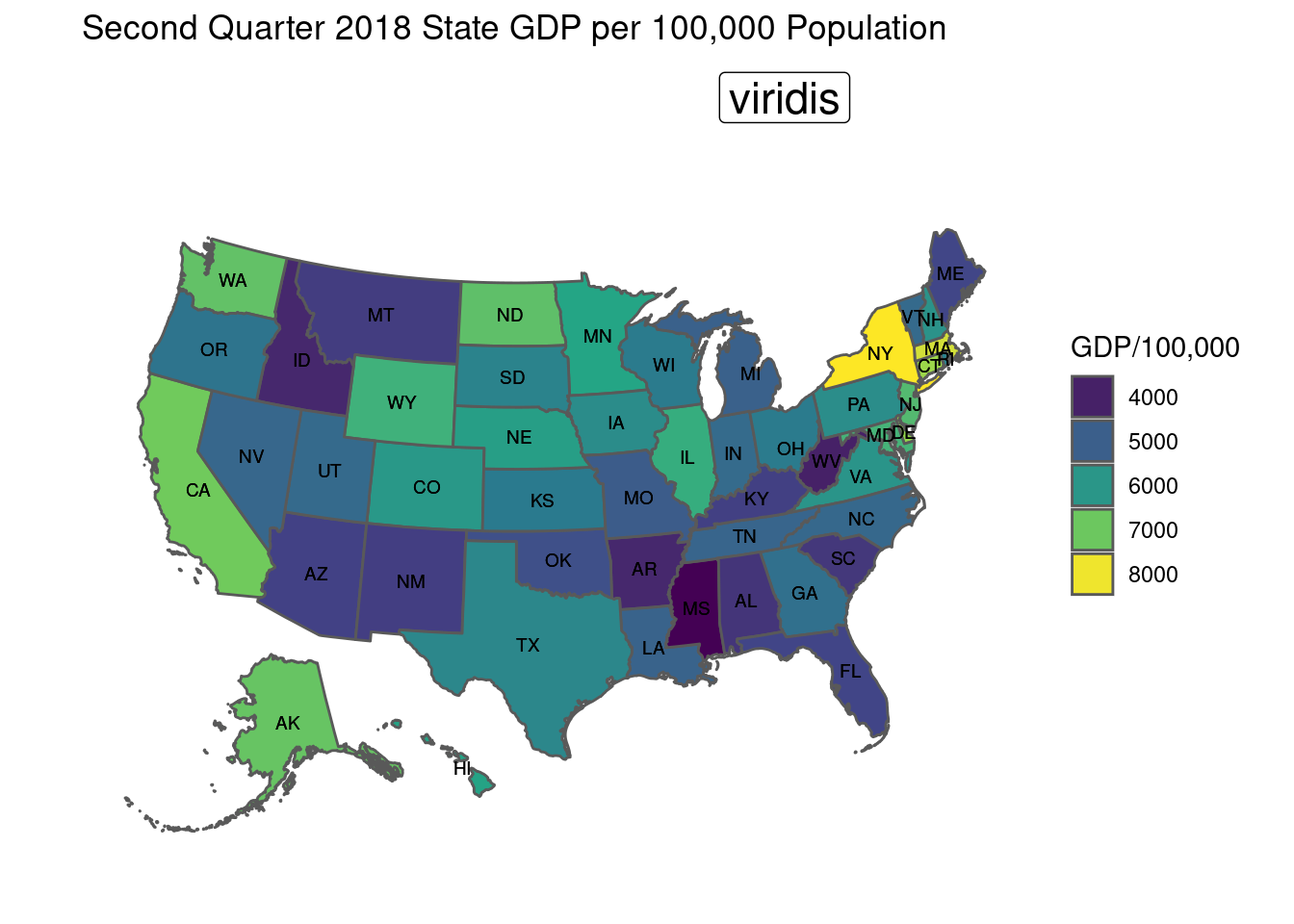
scale_fill_viridis_c(option="viridis")
scale_fill_viridis_c(option="viridis")
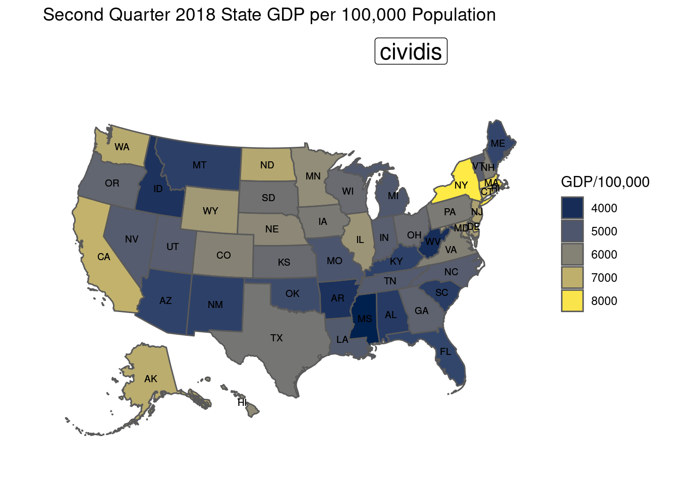
Fortunately, the palette can be muted with an alpha density filter
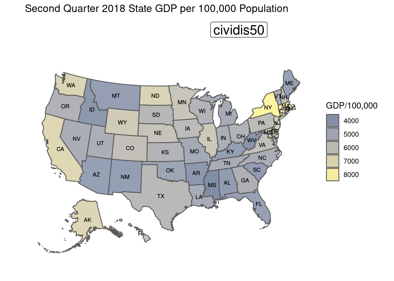
scale_fill_viridis_c(alpha = 0.50, option="cividis")
ggplot’s scale_fill_gradient can also over-ride default colors
The signature of scale_fill_gradient is
scale_fill_gradient(..., low = "#132B43", high = "#56B1F7", space = "Lab", na.value = "grey50", guide = "colourbar", aesthetics = "fill")
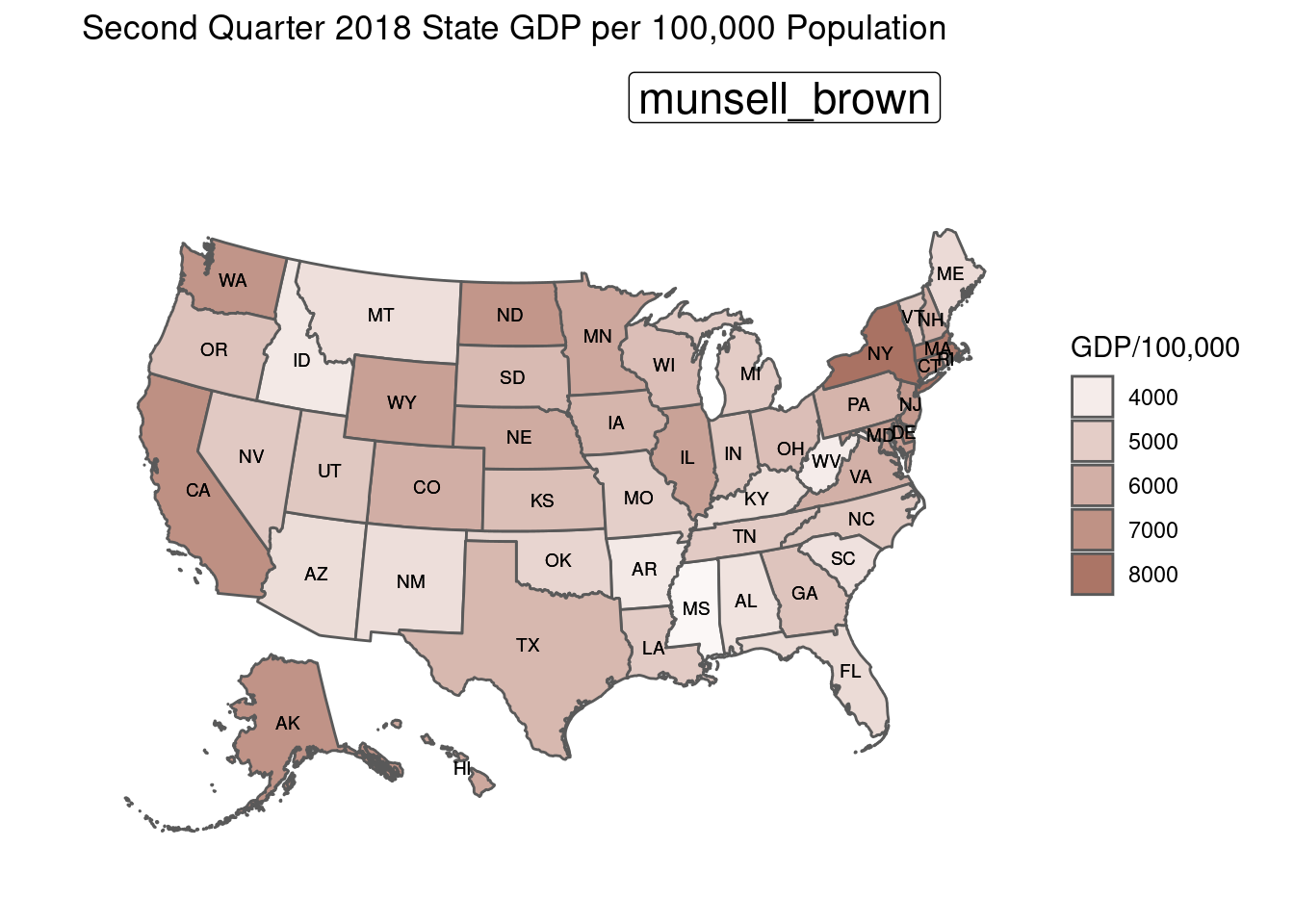
in the blue range. You can adjust that with the arguments to low and high. The following example uses #FBF7F6 and #A97263.
How did I come up with those particular values?
library(munsell)
show_col(seq_gradient_pal("white", mnsl("10R 4/6"))(x))(seq(0, 1, length.out = 25)))
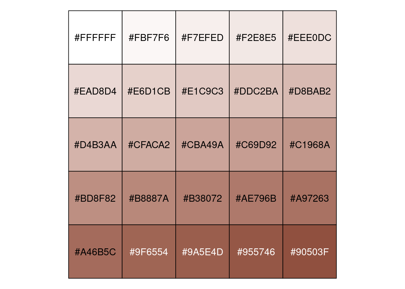
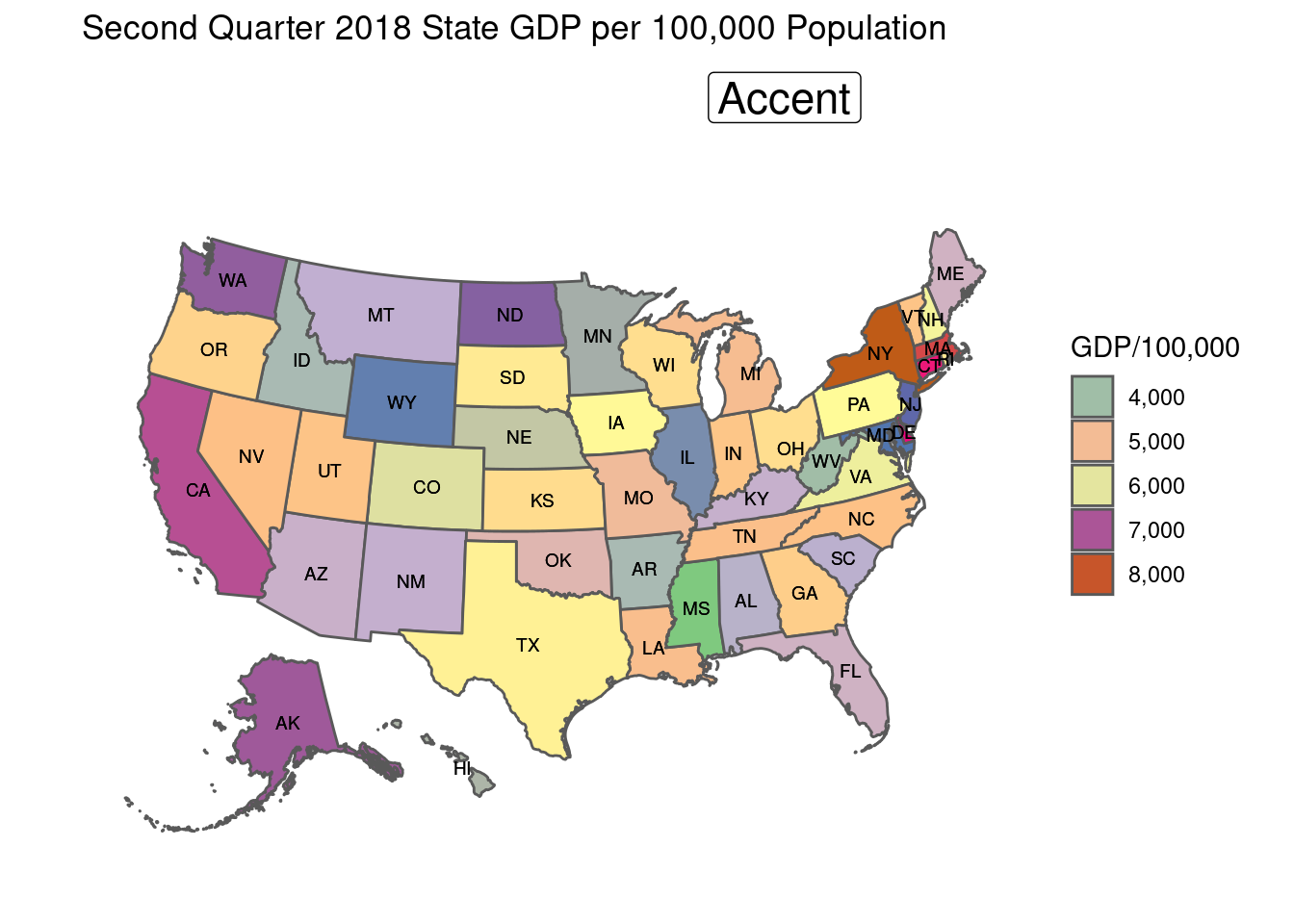
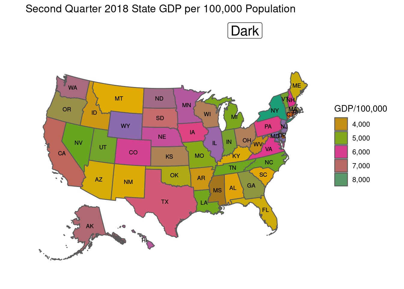
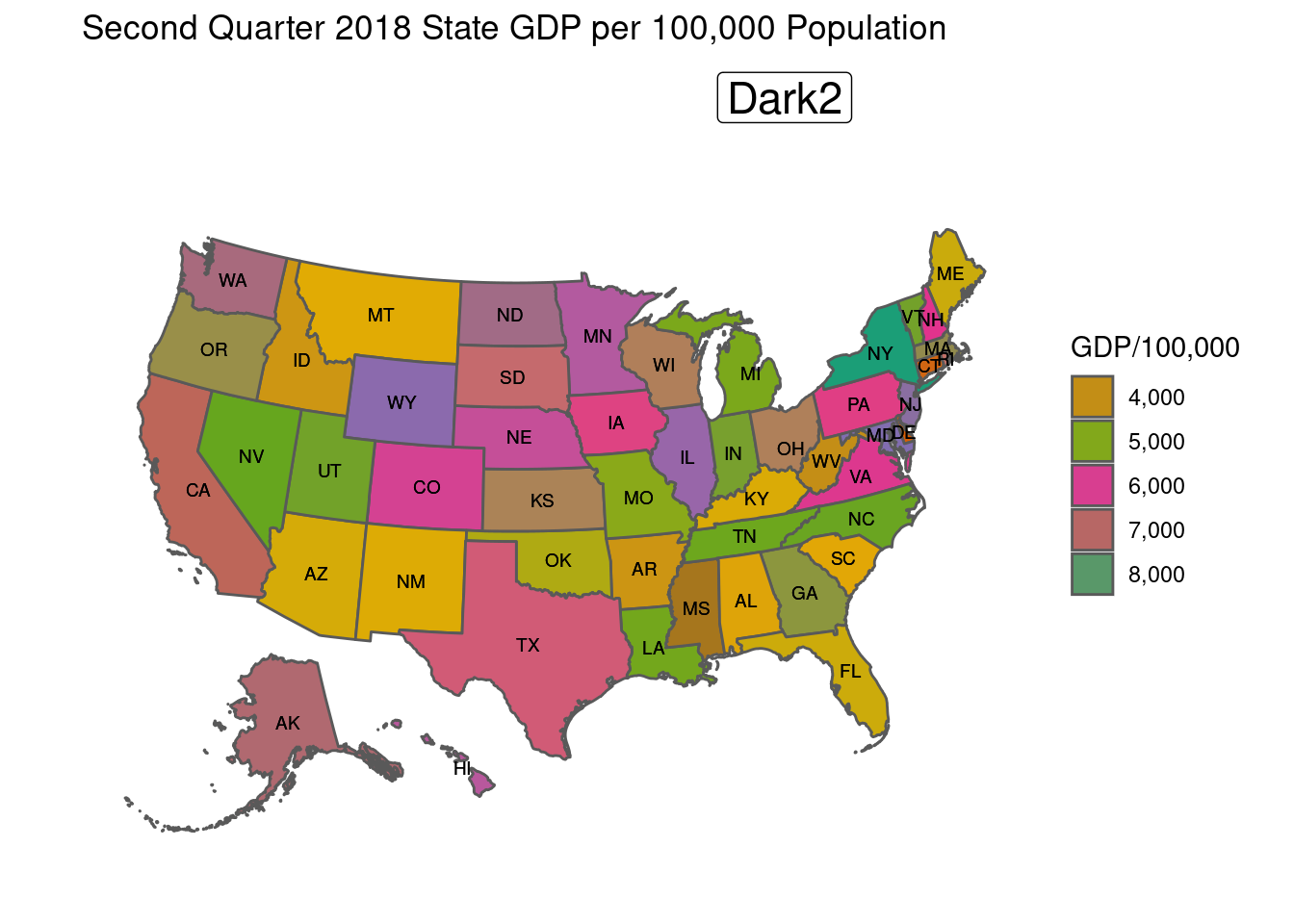
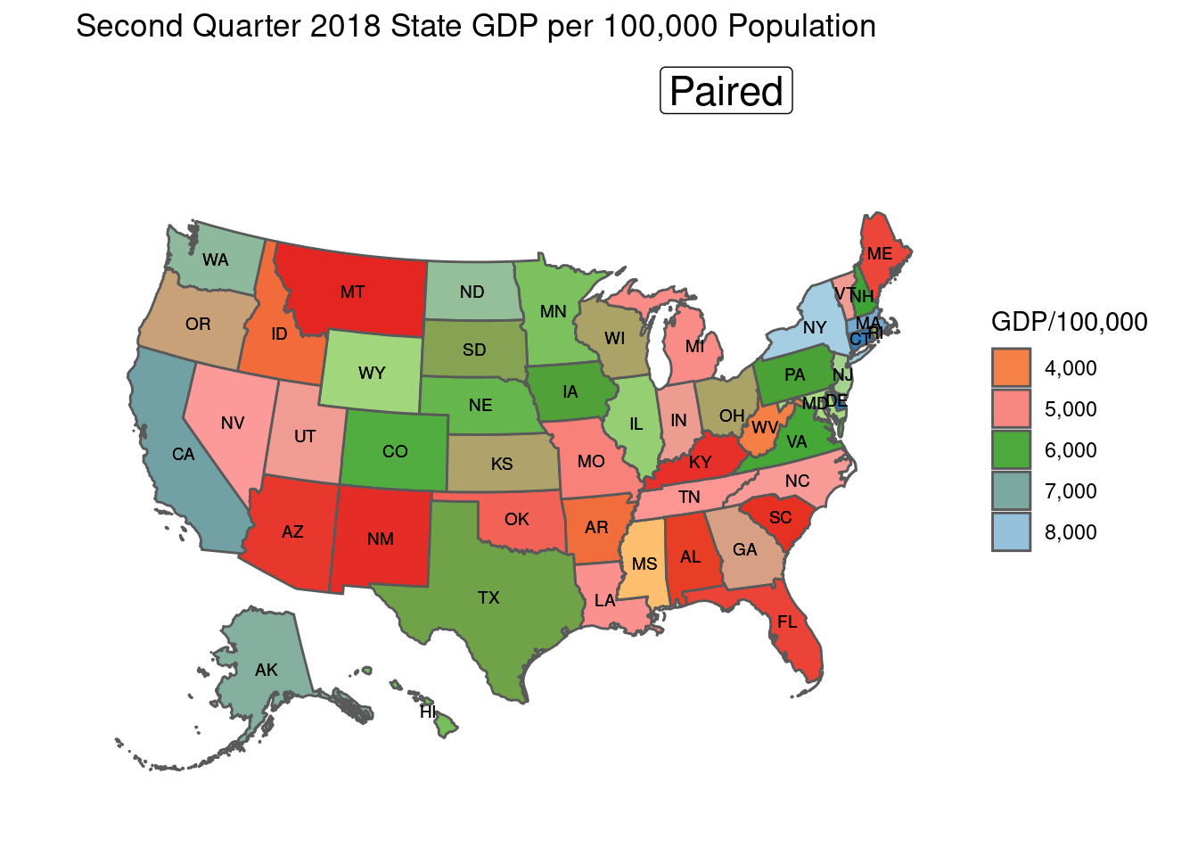
This approach, and other do-it-yourself color palette selection approaches can become a time sink.See R color cheatsheet A better approach is to have a selection of pre-made color cards, and try them out until one of them highlights the differences you are trying to show.
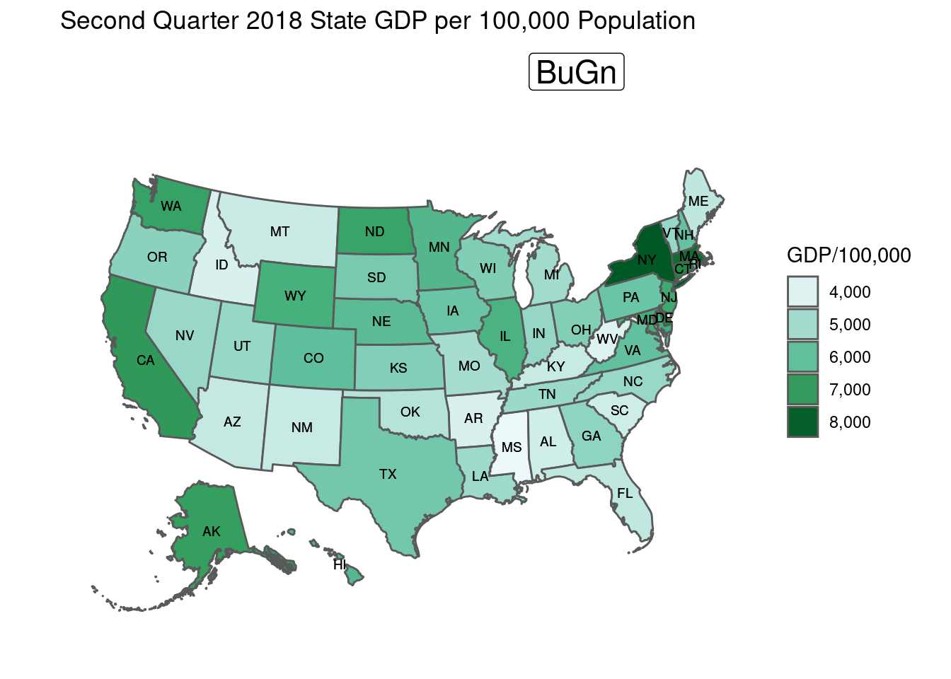
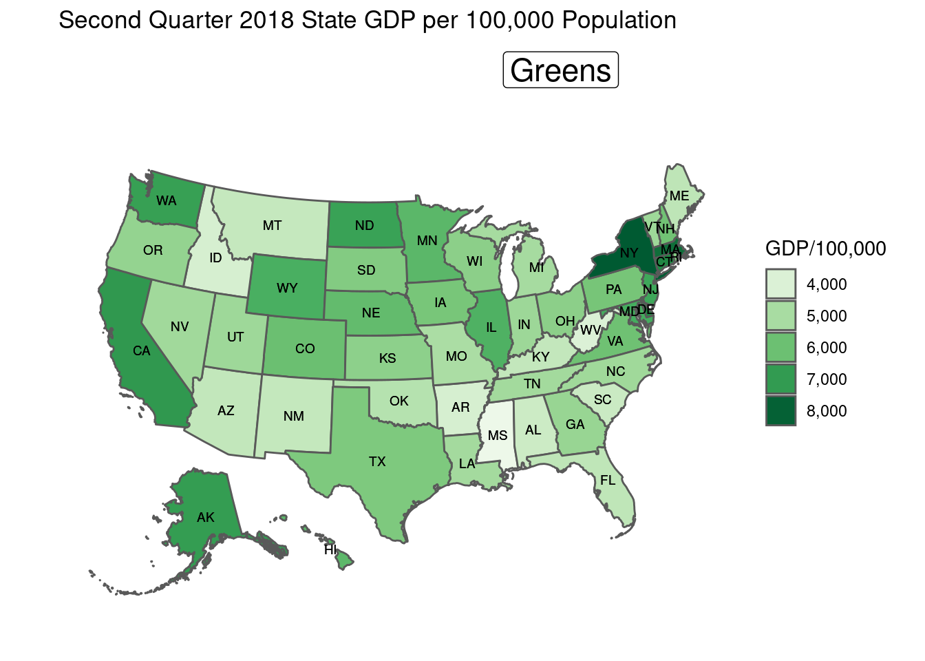
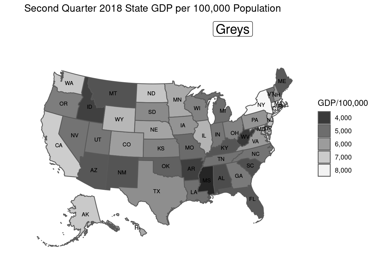
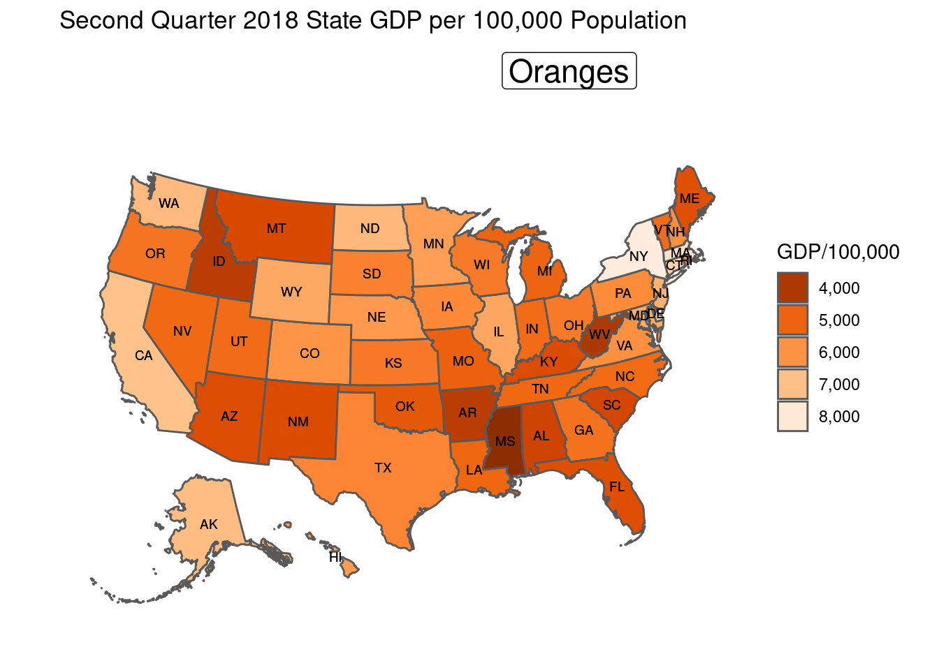
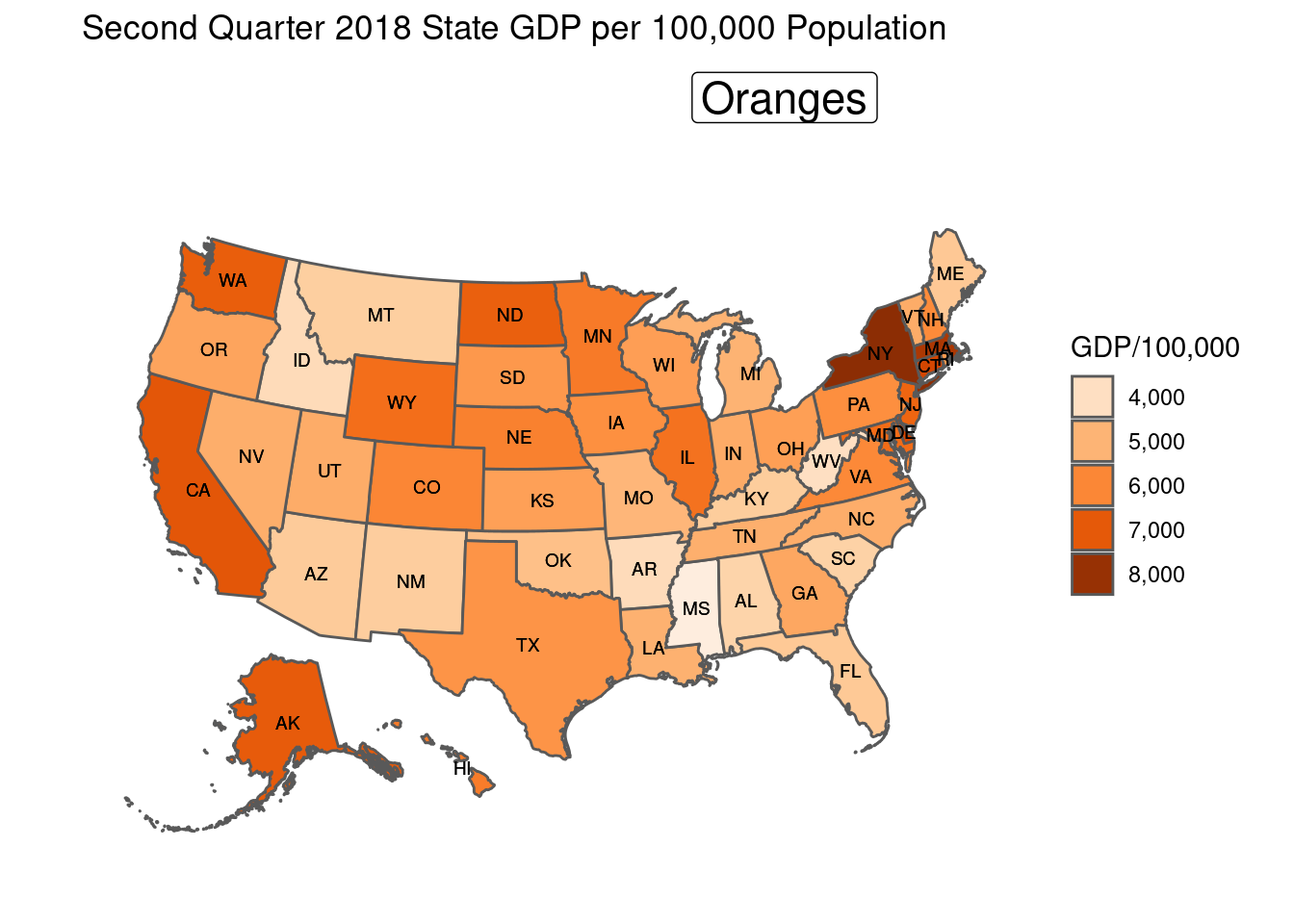
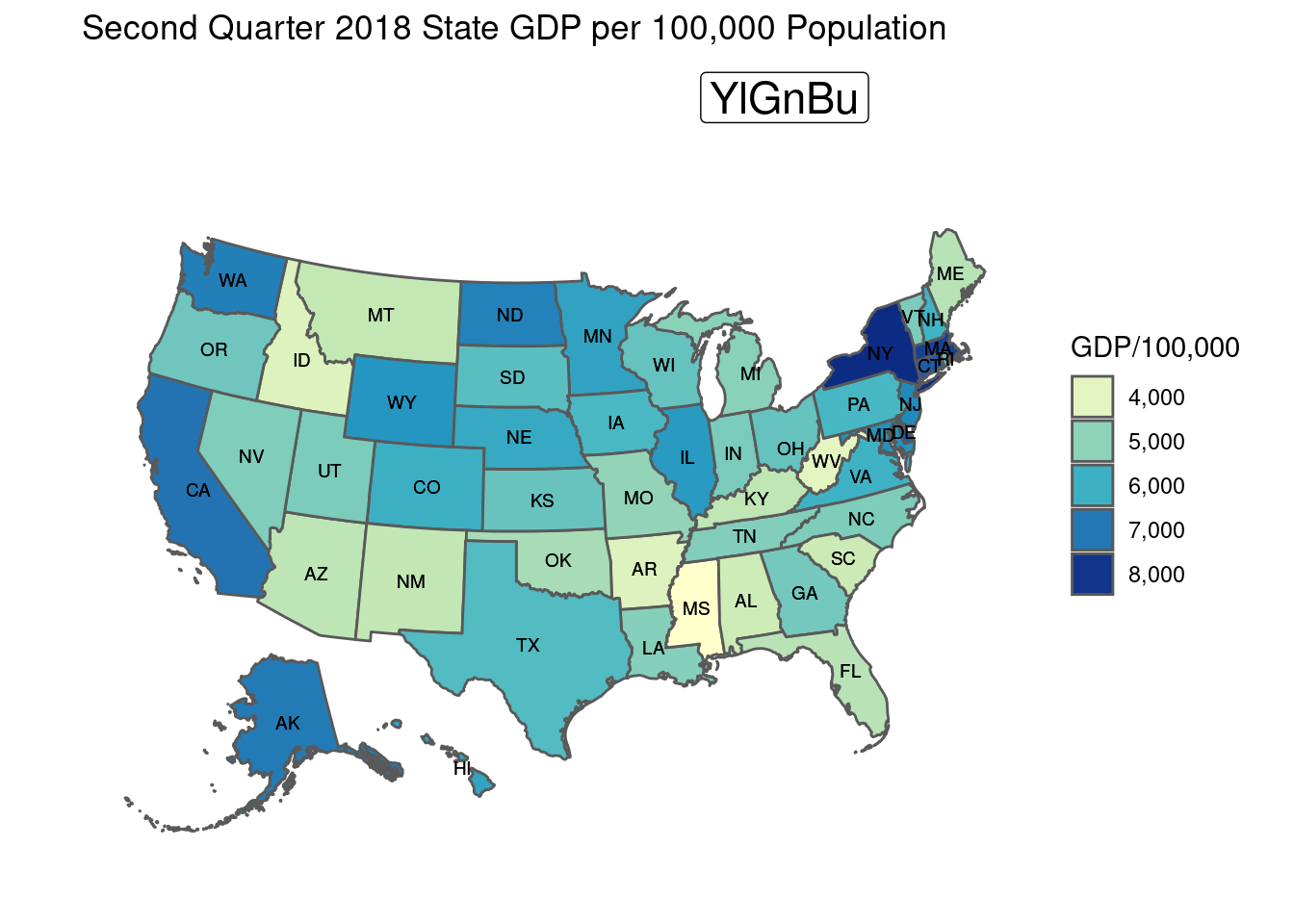
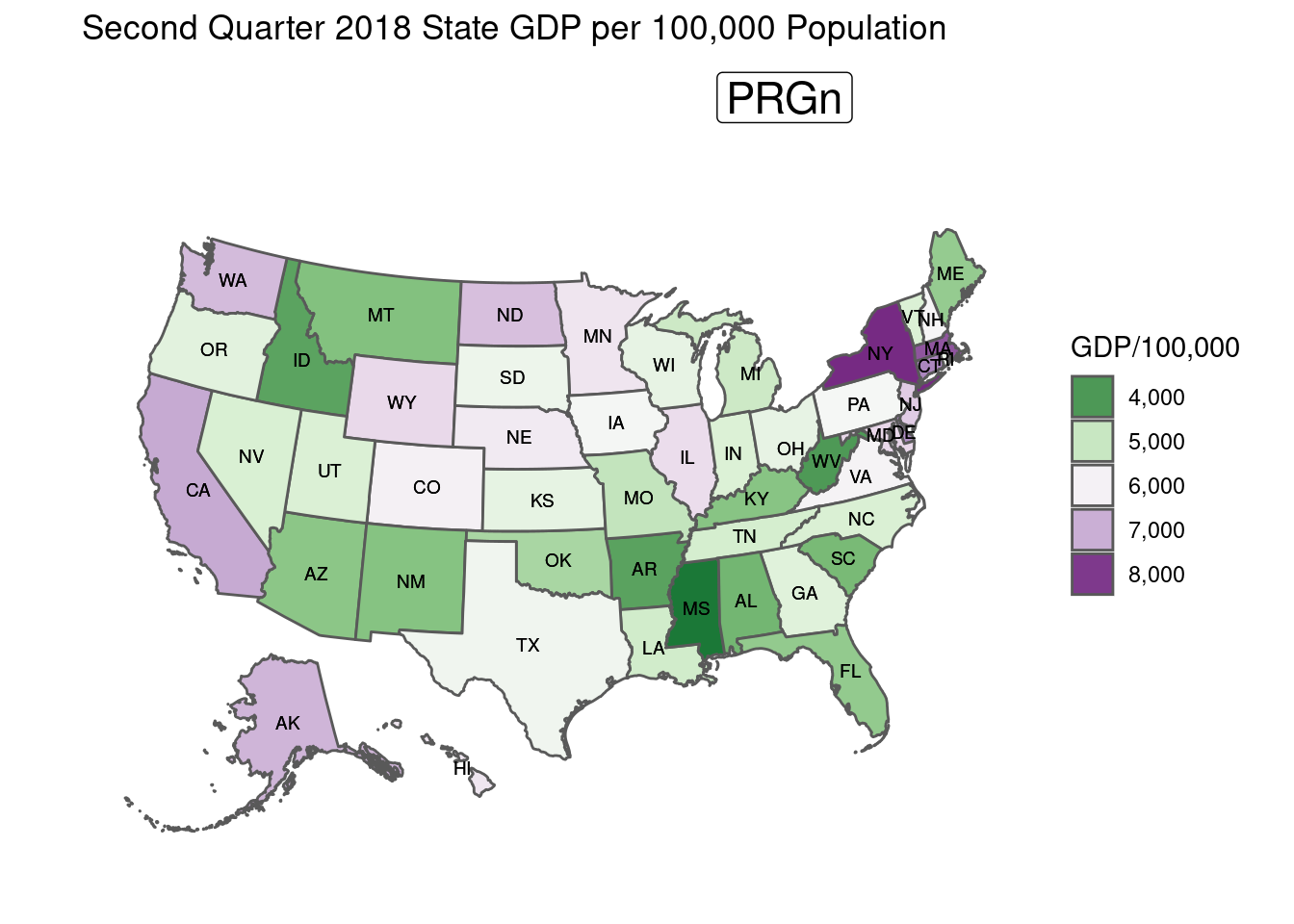
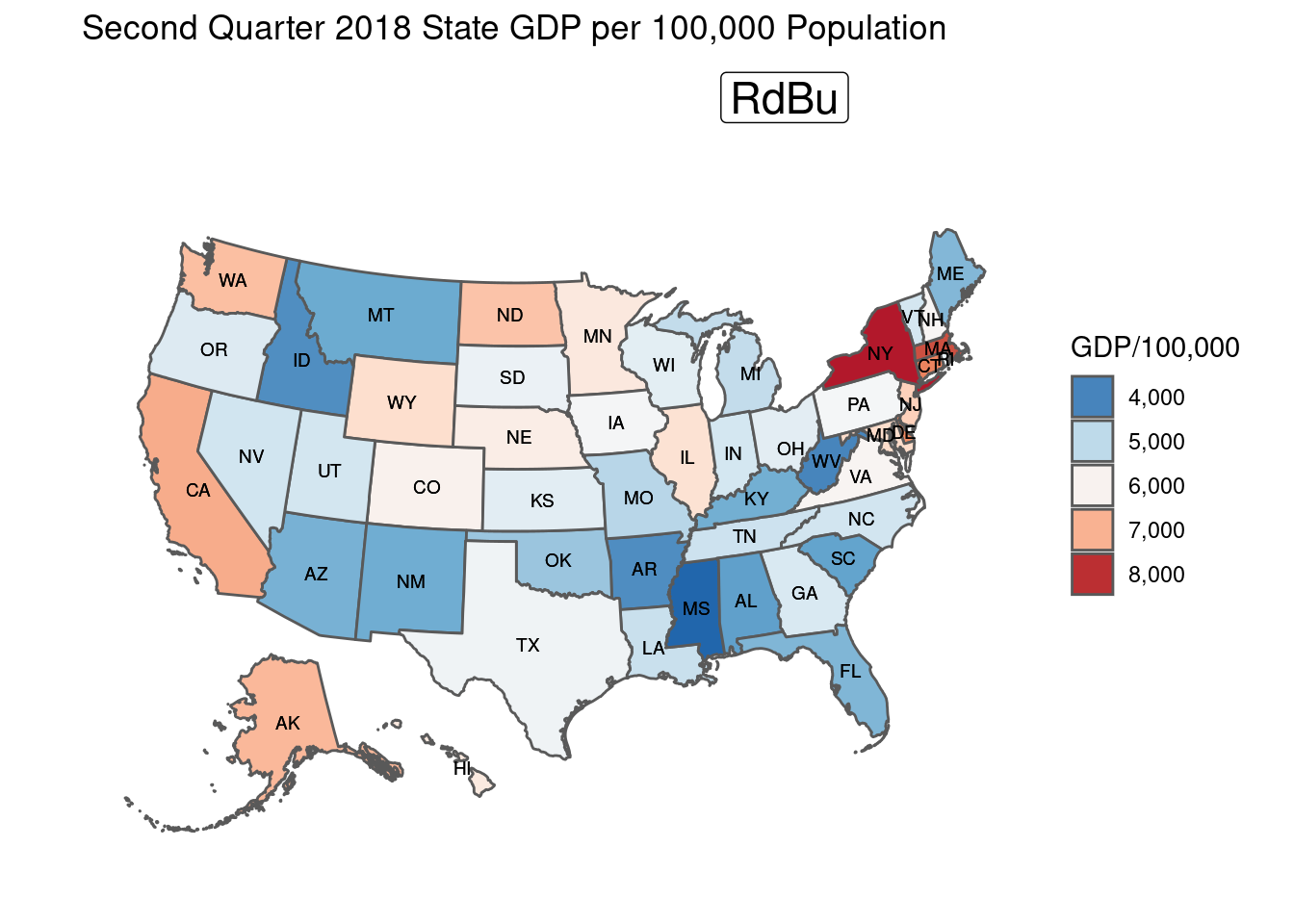
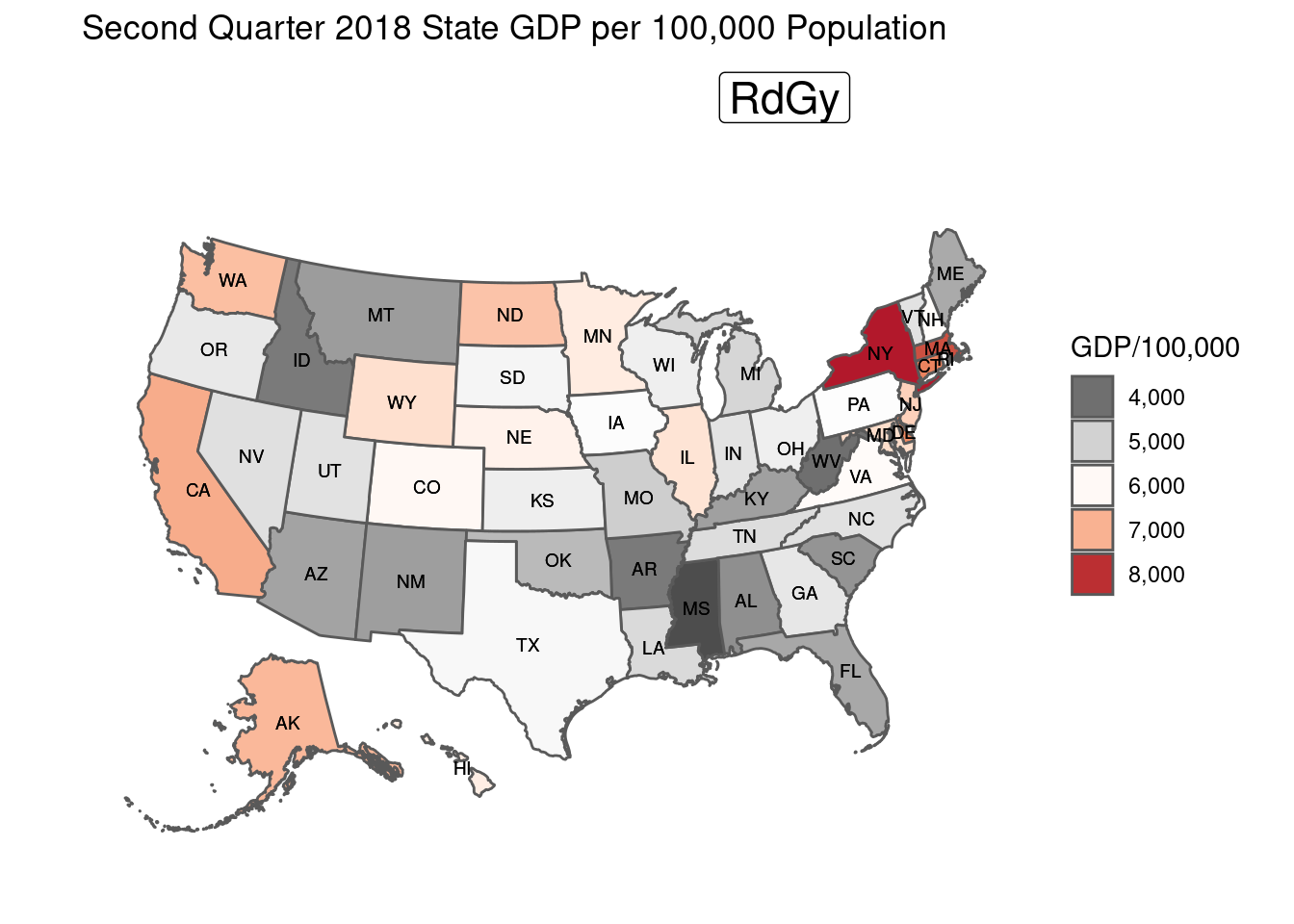
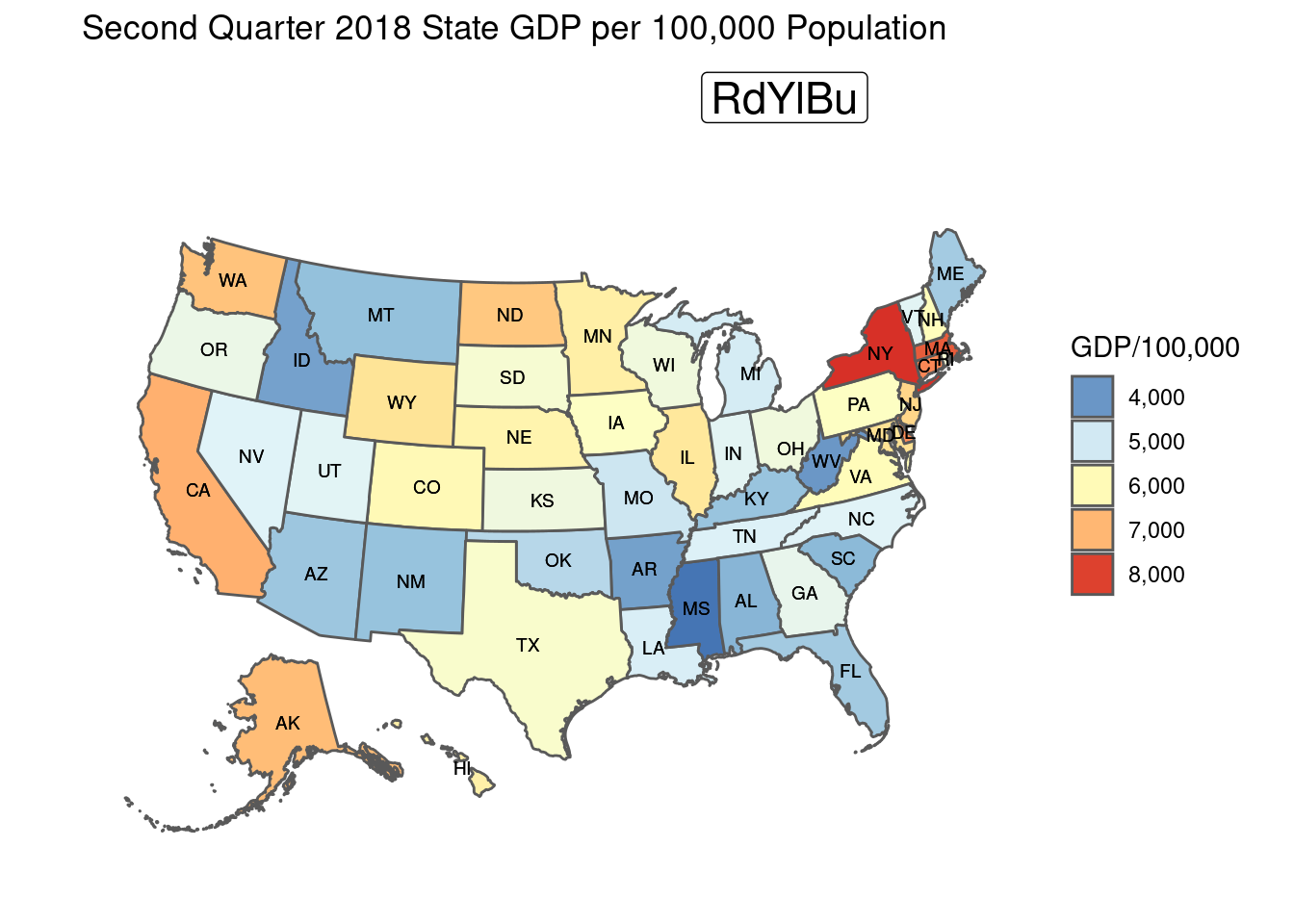
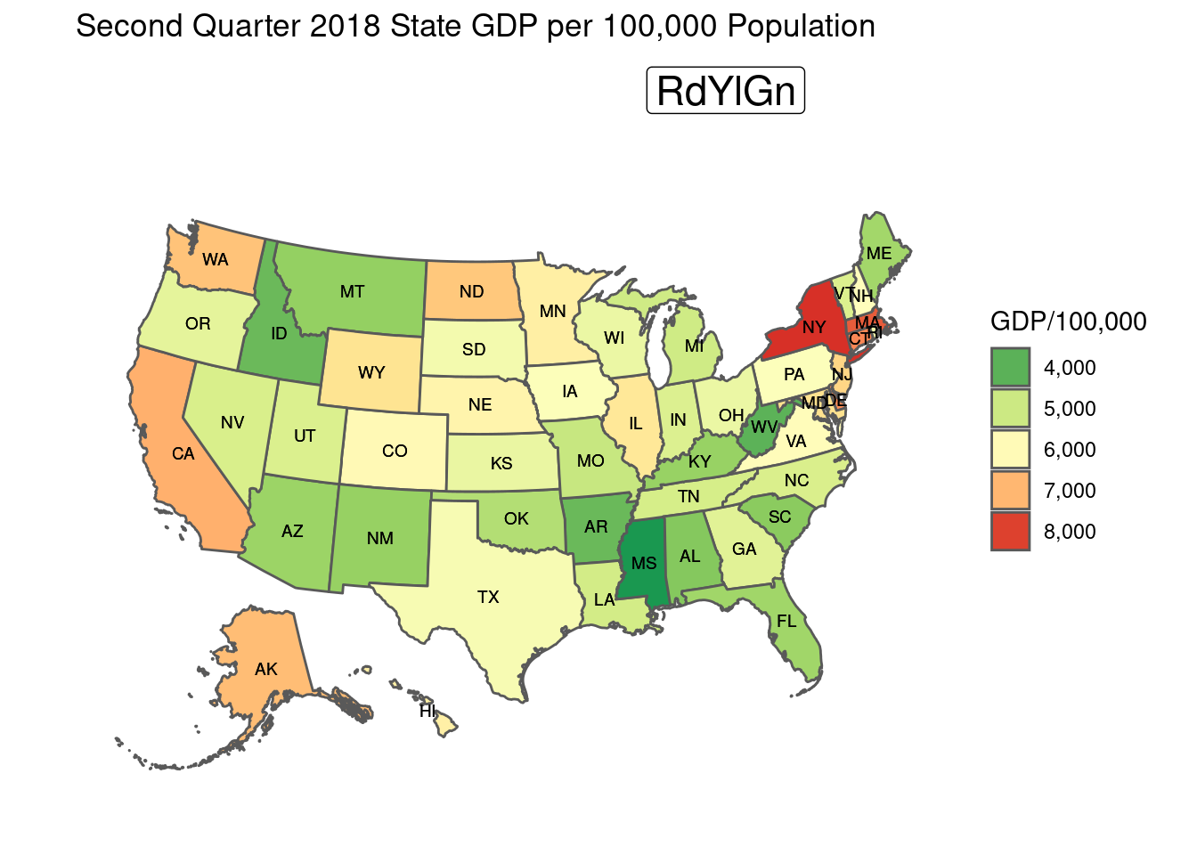
RColorBrewer
This set of palettes plays well with ggplot and should answer most needs.

RColorBrewer
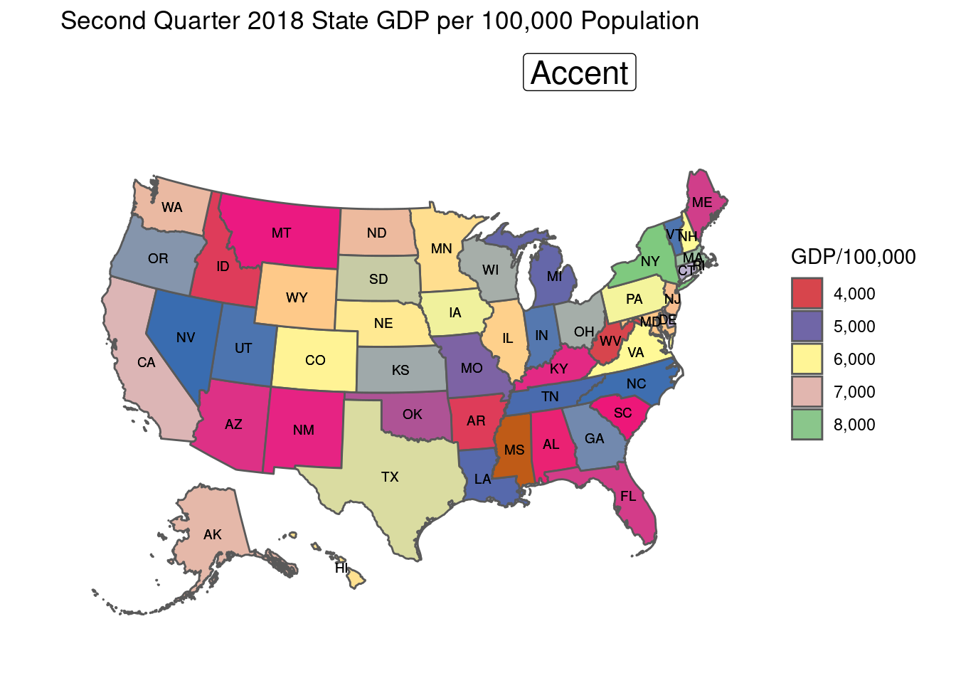
The three sections are for sequential (i.e., continuous), divergent (a neutral color in the center progressing toward more intense colors in both direction) or qualitative, for discrete data but coercible into continuous data.
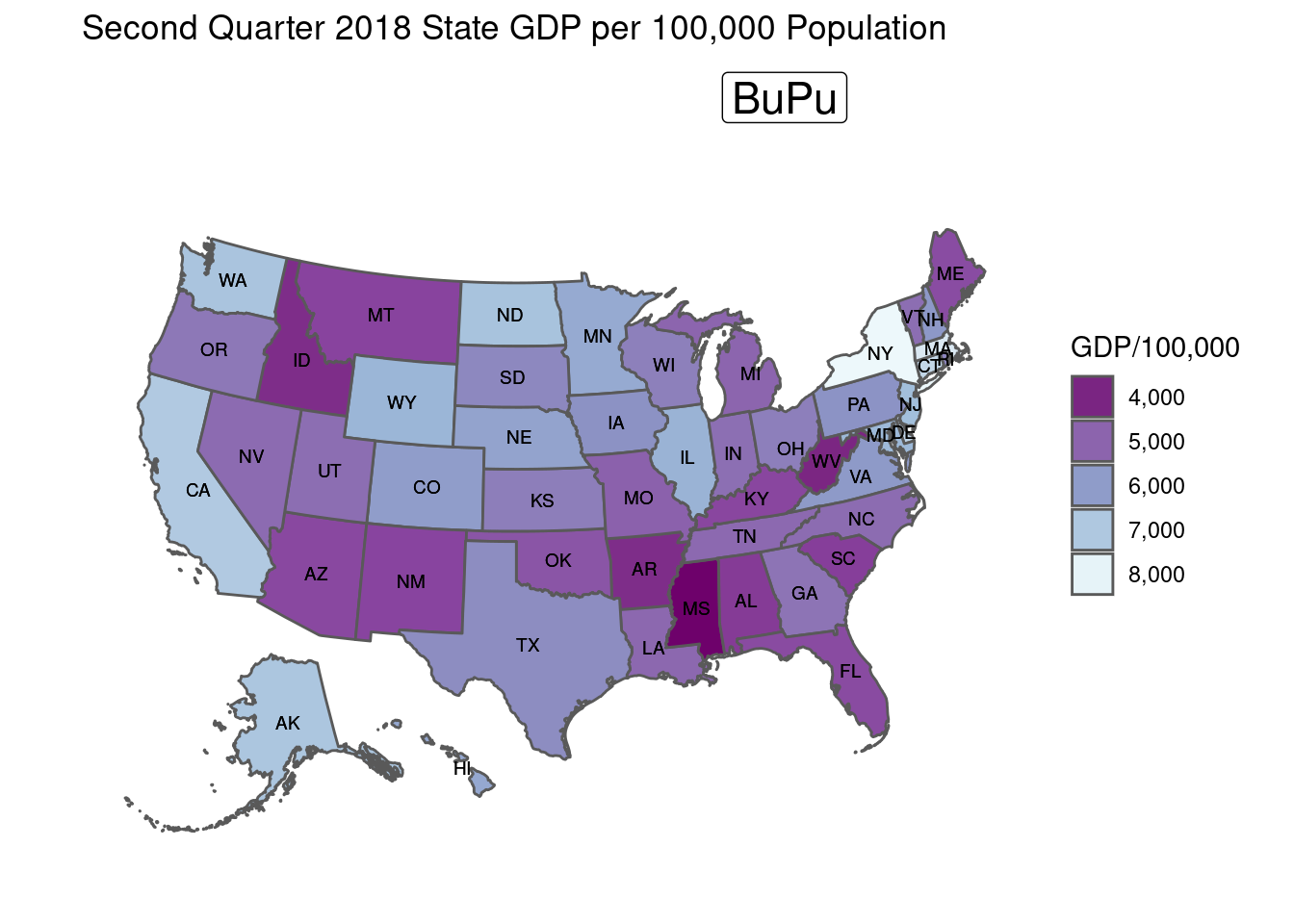
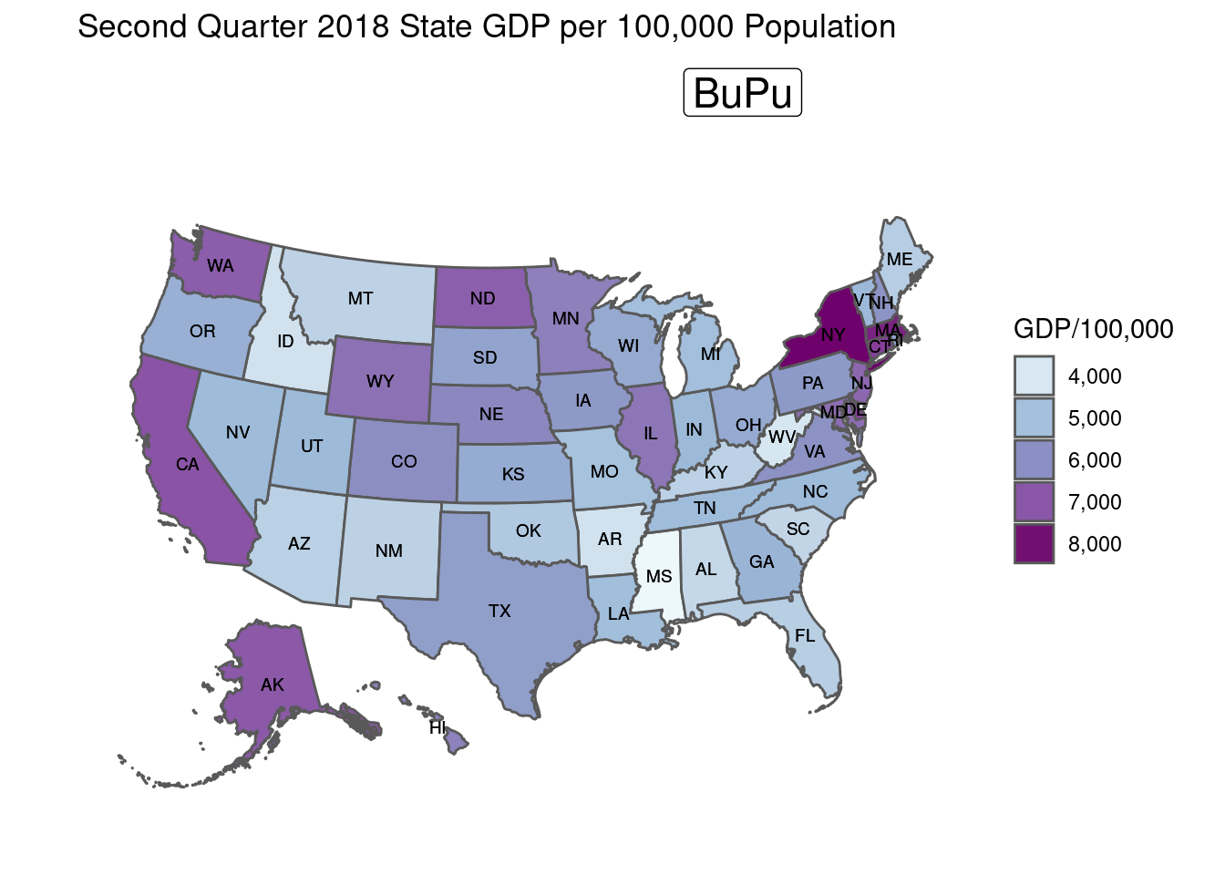
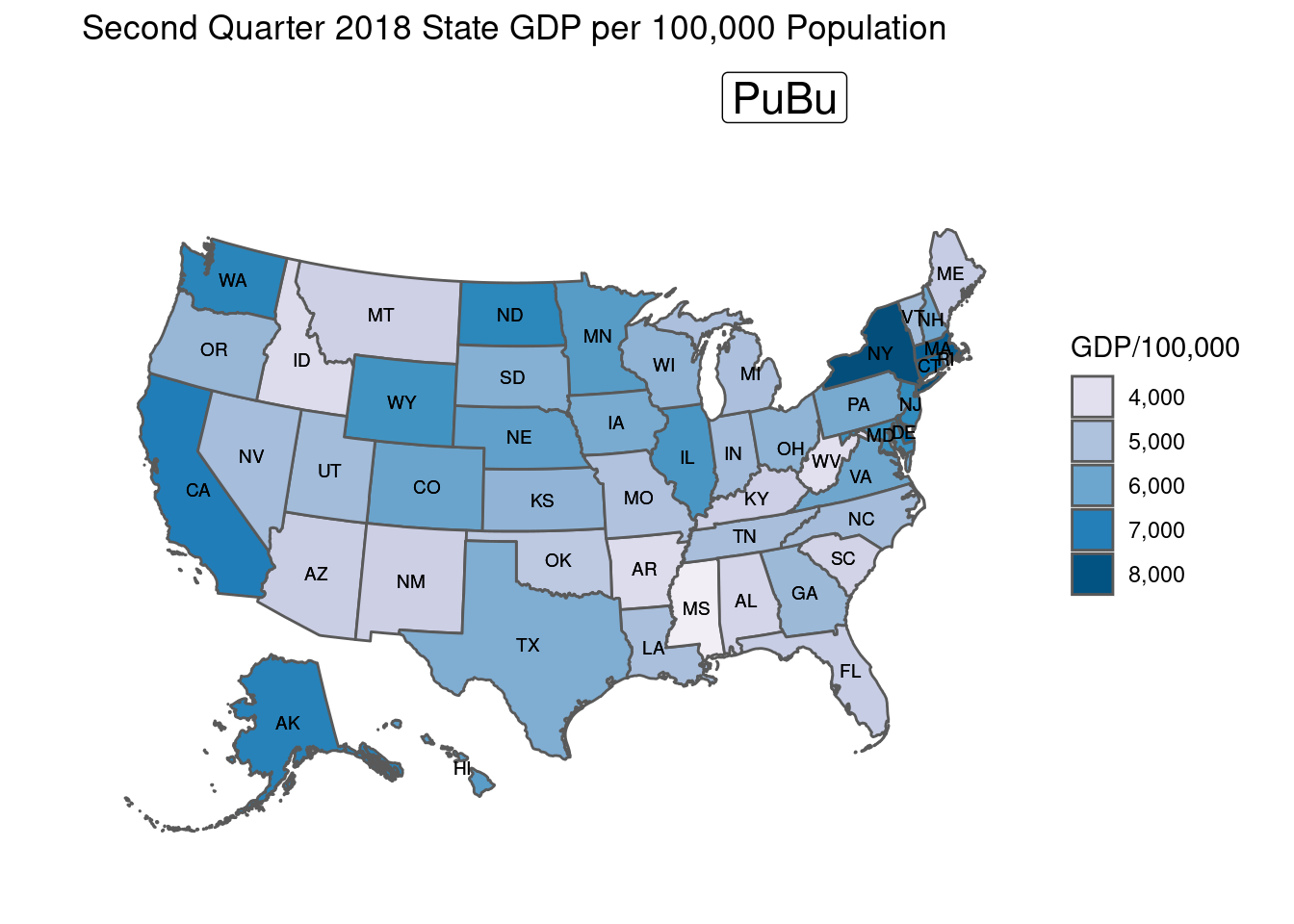
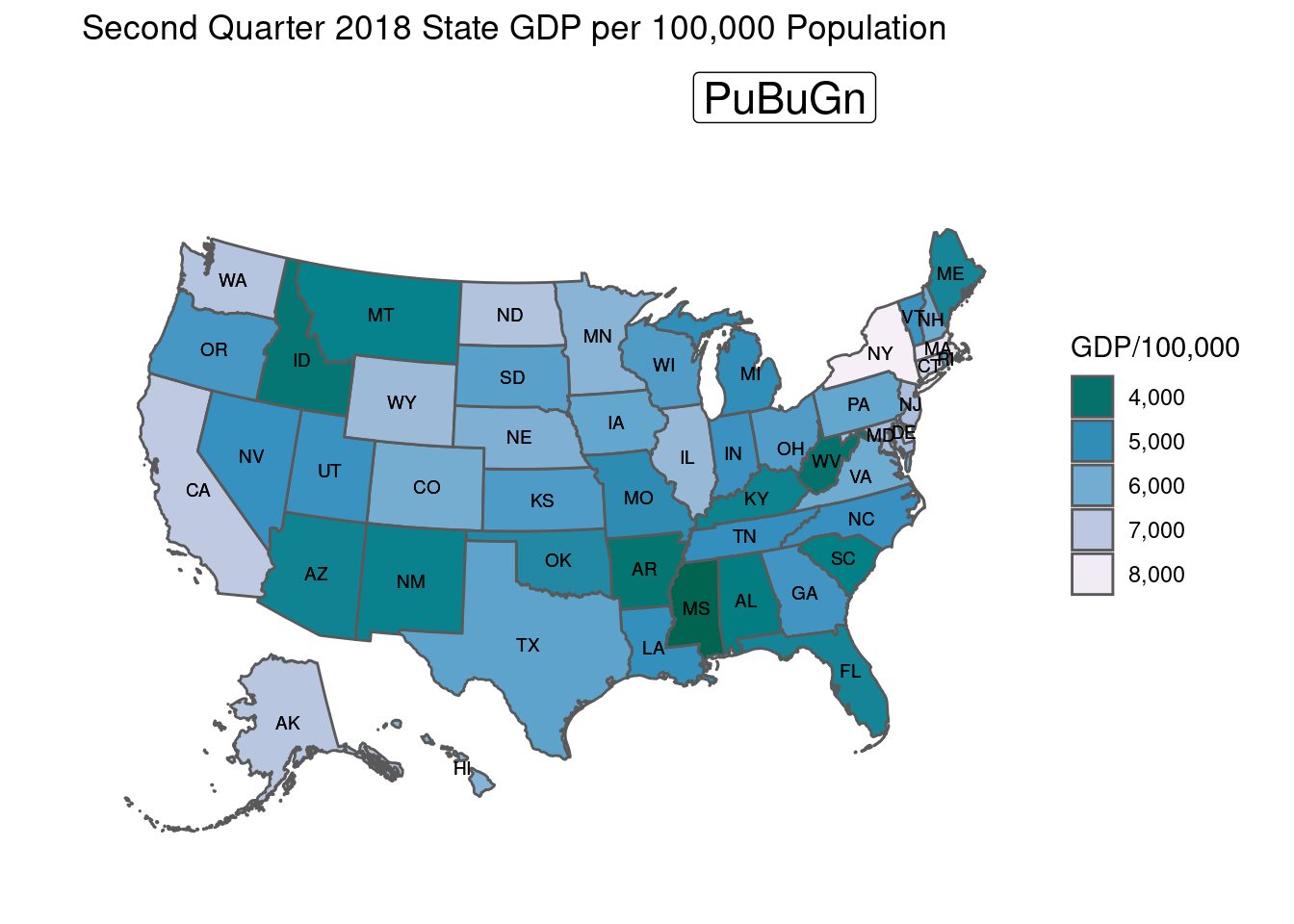
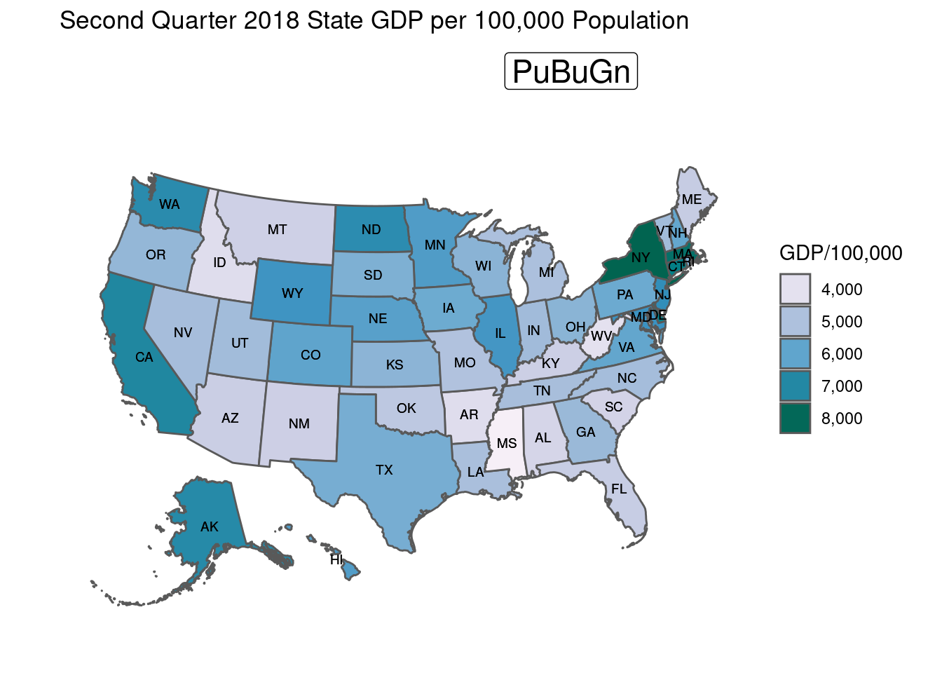
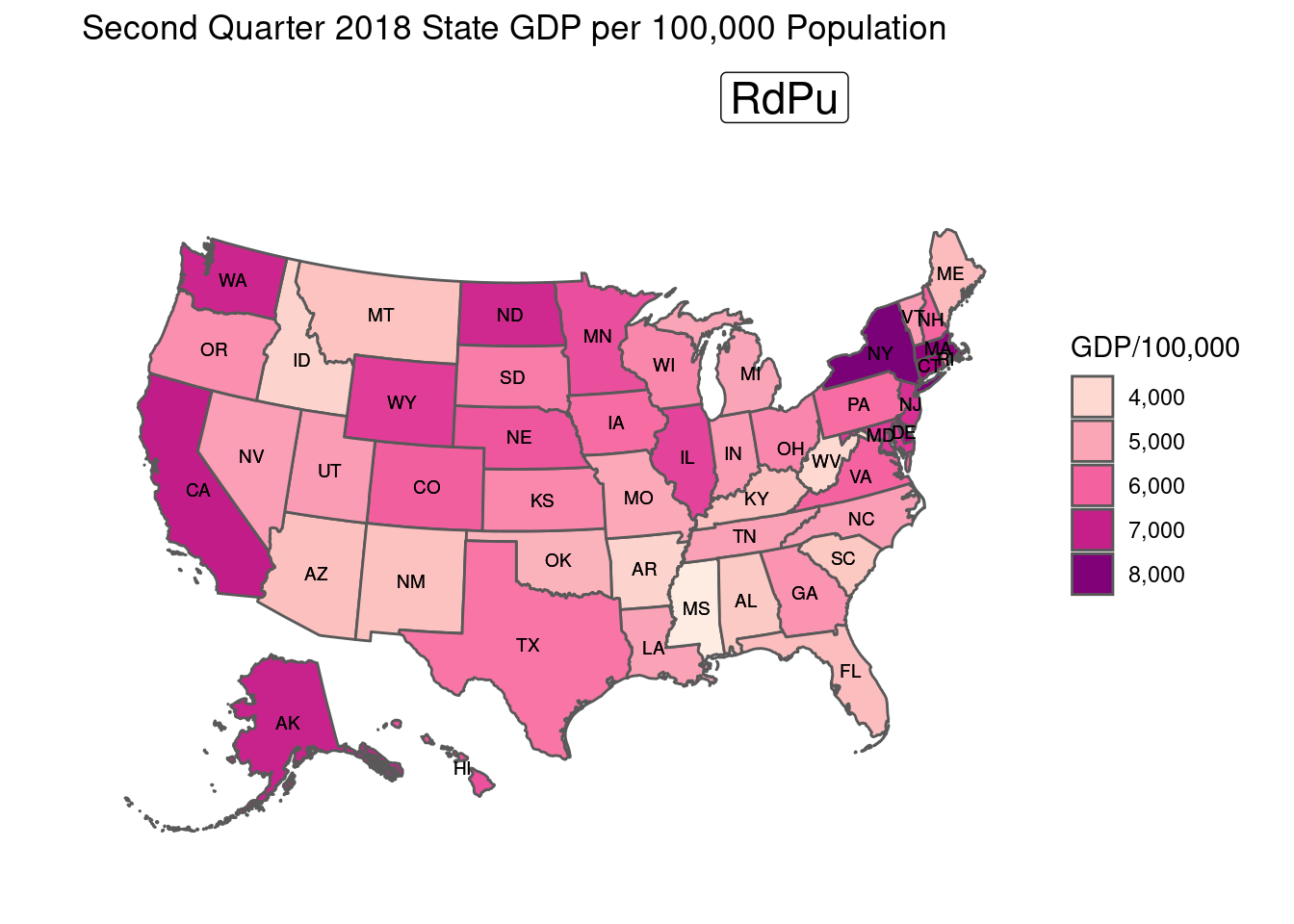
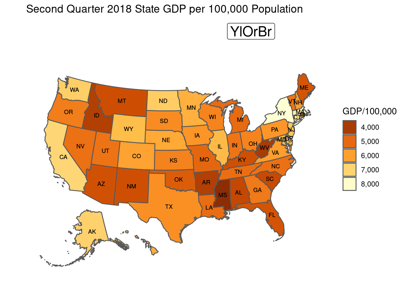
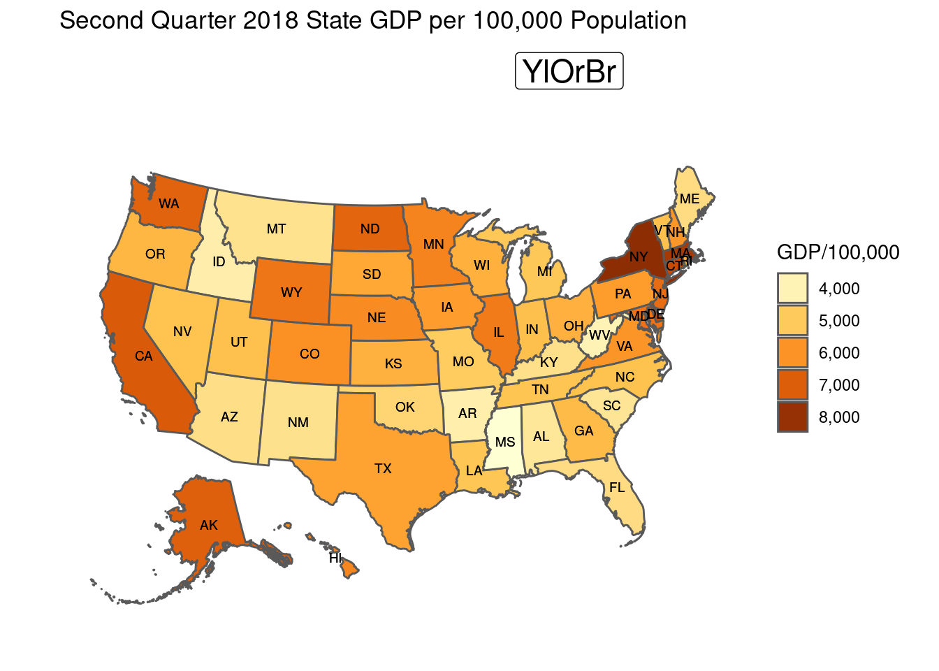
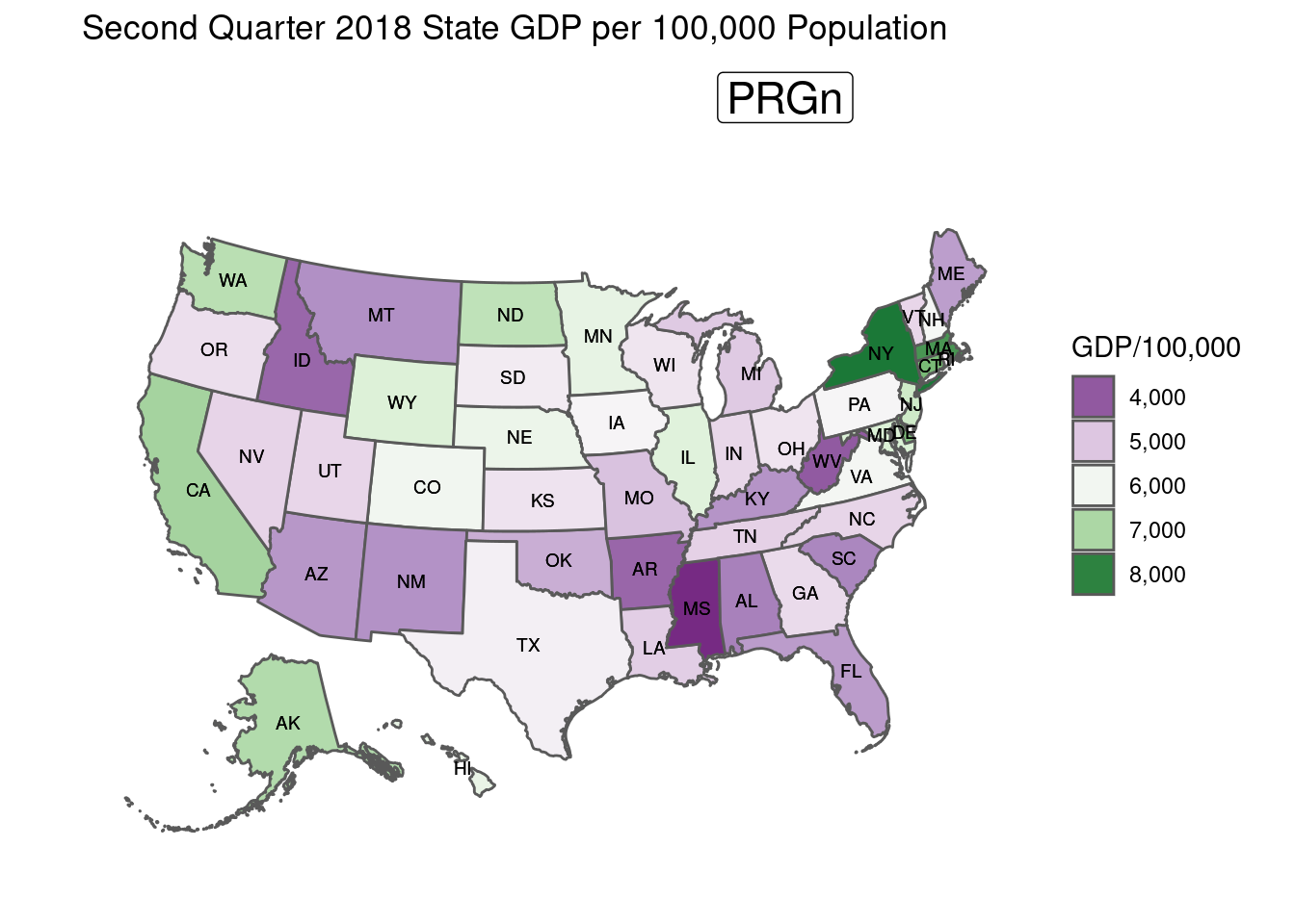
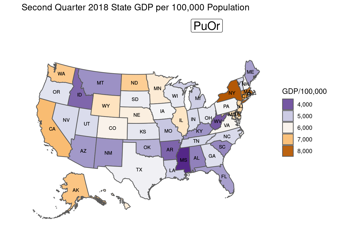
Through ggplot’s scale_colour_distiller function, any of these can be smoothly interpolated into a six-interval scale.
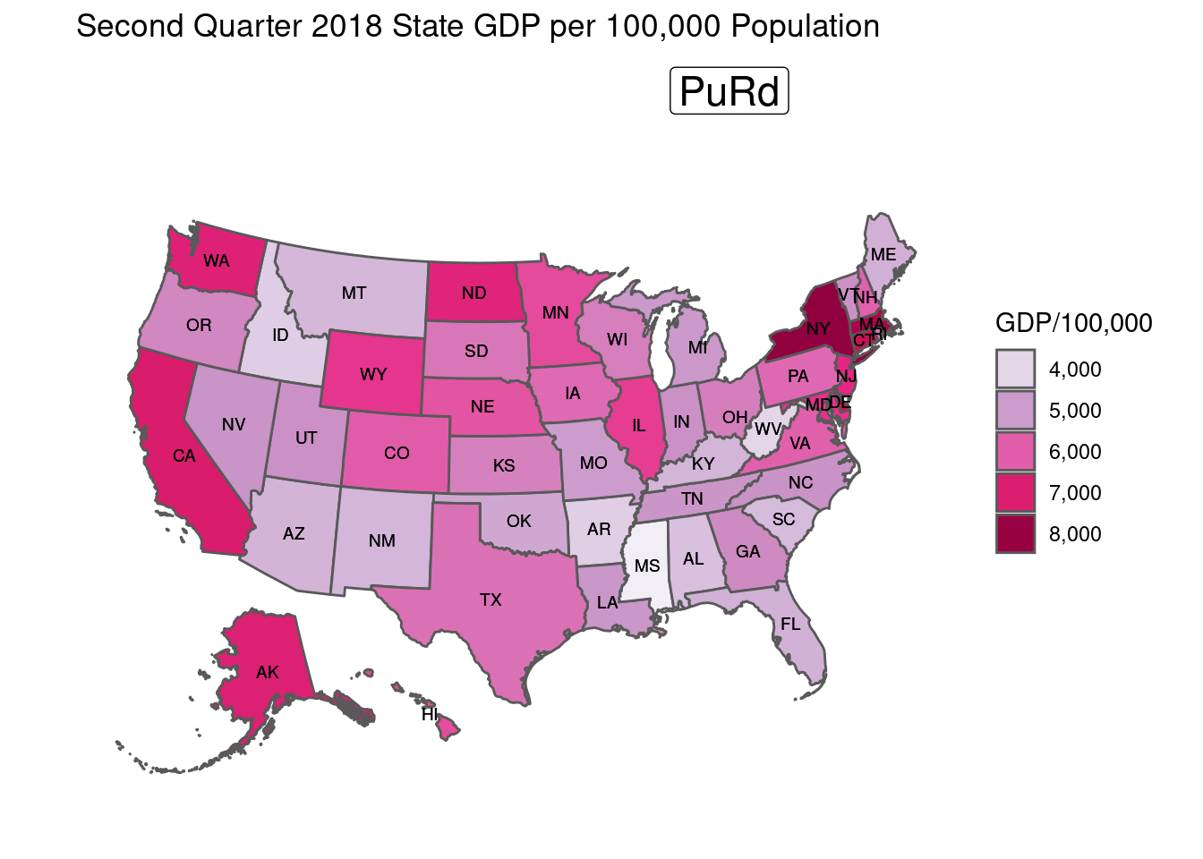
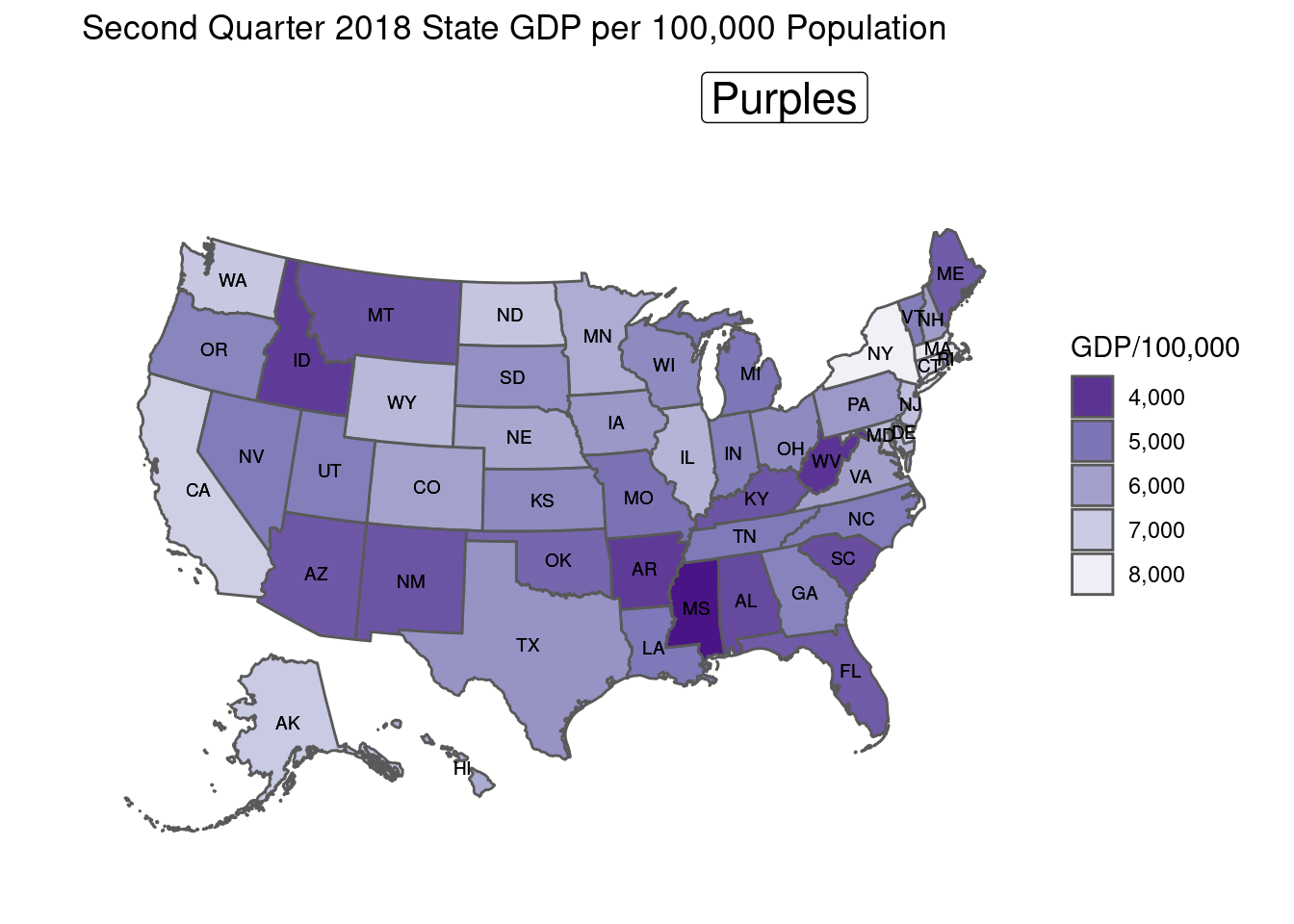
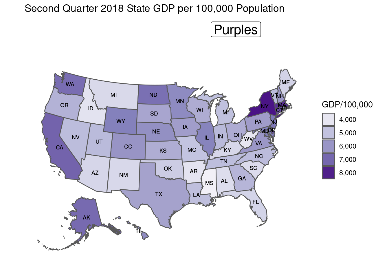
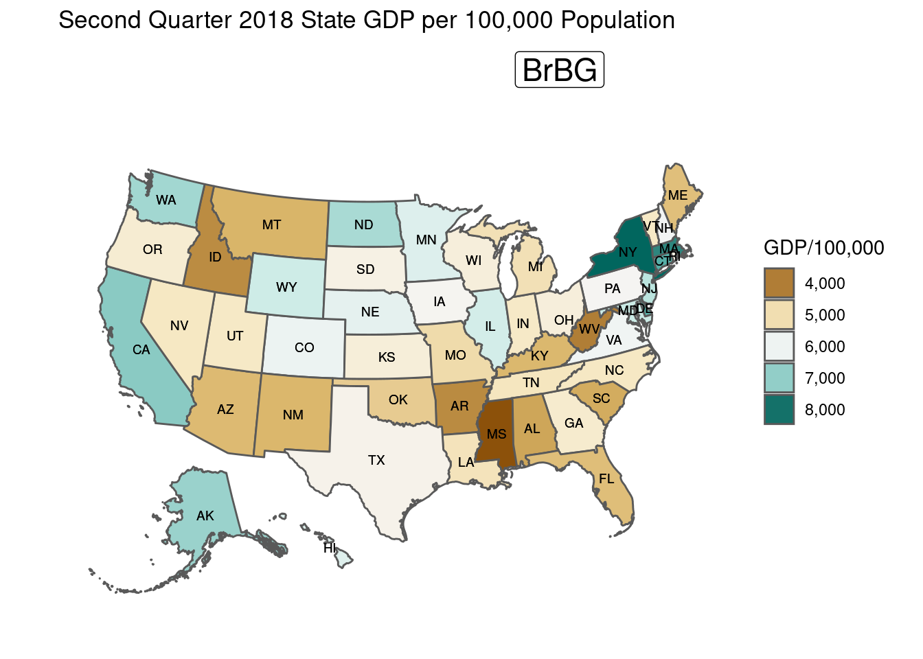
All of the scales can be flipped, working from left-to-right on the palette or from right-to-left. Direction is indicated by direction = -1 or direction = 1.
Color abbreviations:
- Yl = Yellow
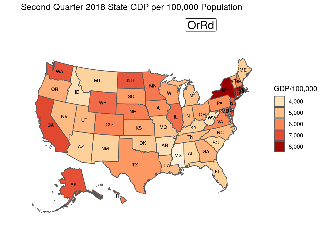
- Or = Orange
- Rd = Red
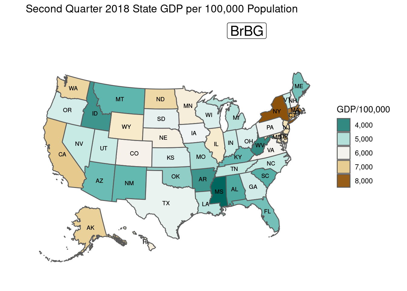
- Br = Brown
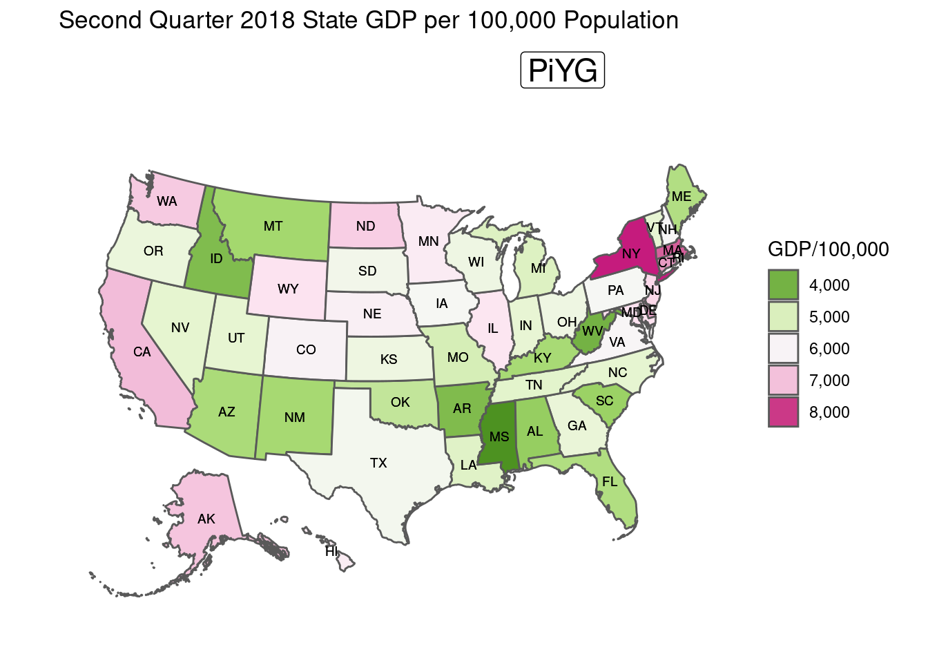
- Gn = Green
- Pu = Purple
- Bu = Blue
There are also:
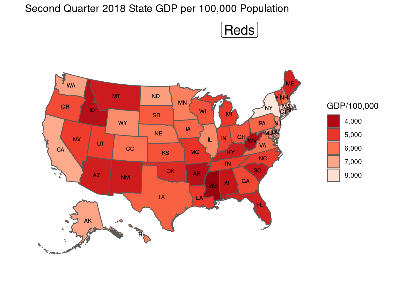
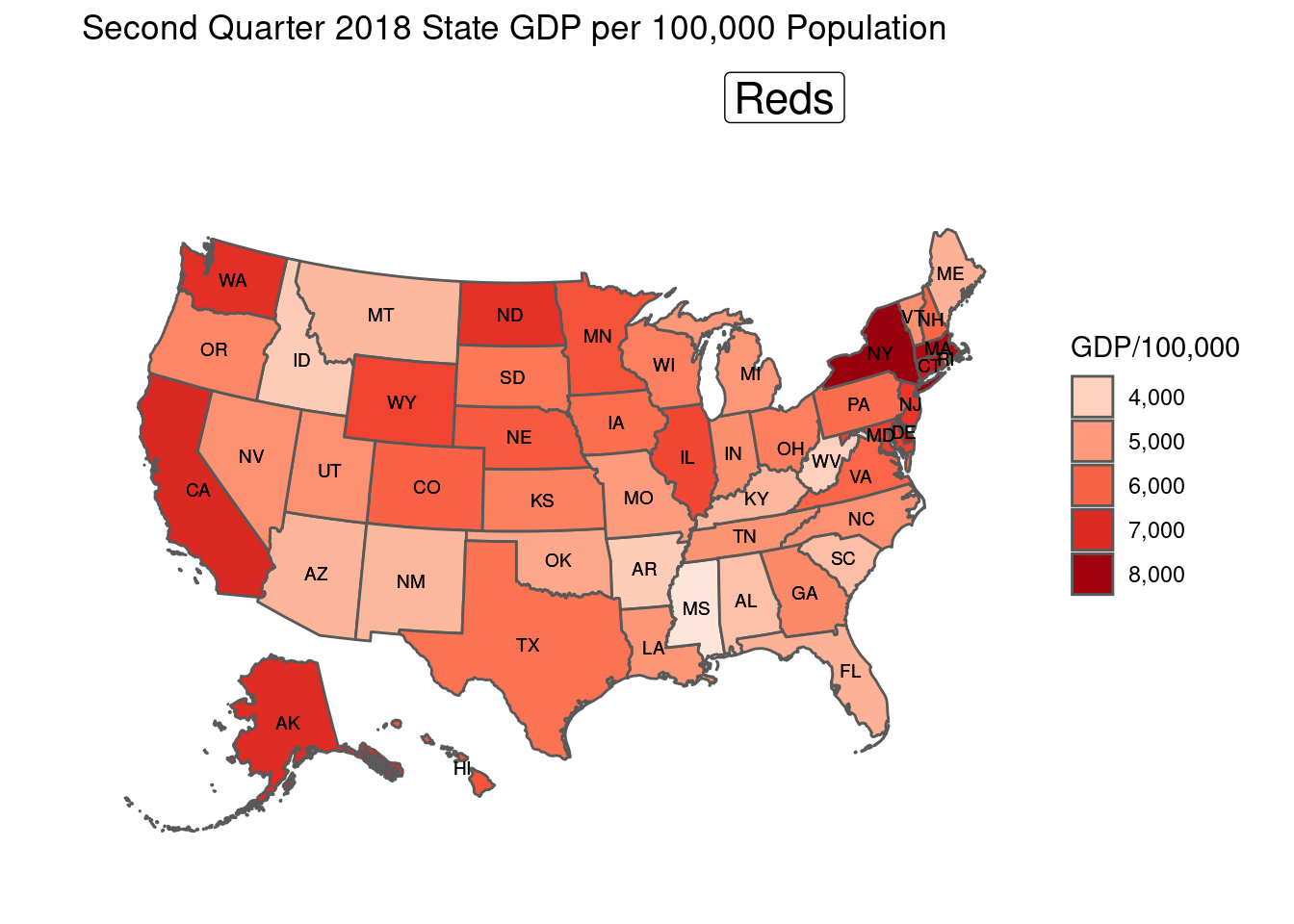
- Reds
- Oranges
- Greys
- Greens
- Blues
The signature for scale_colour_distiller is
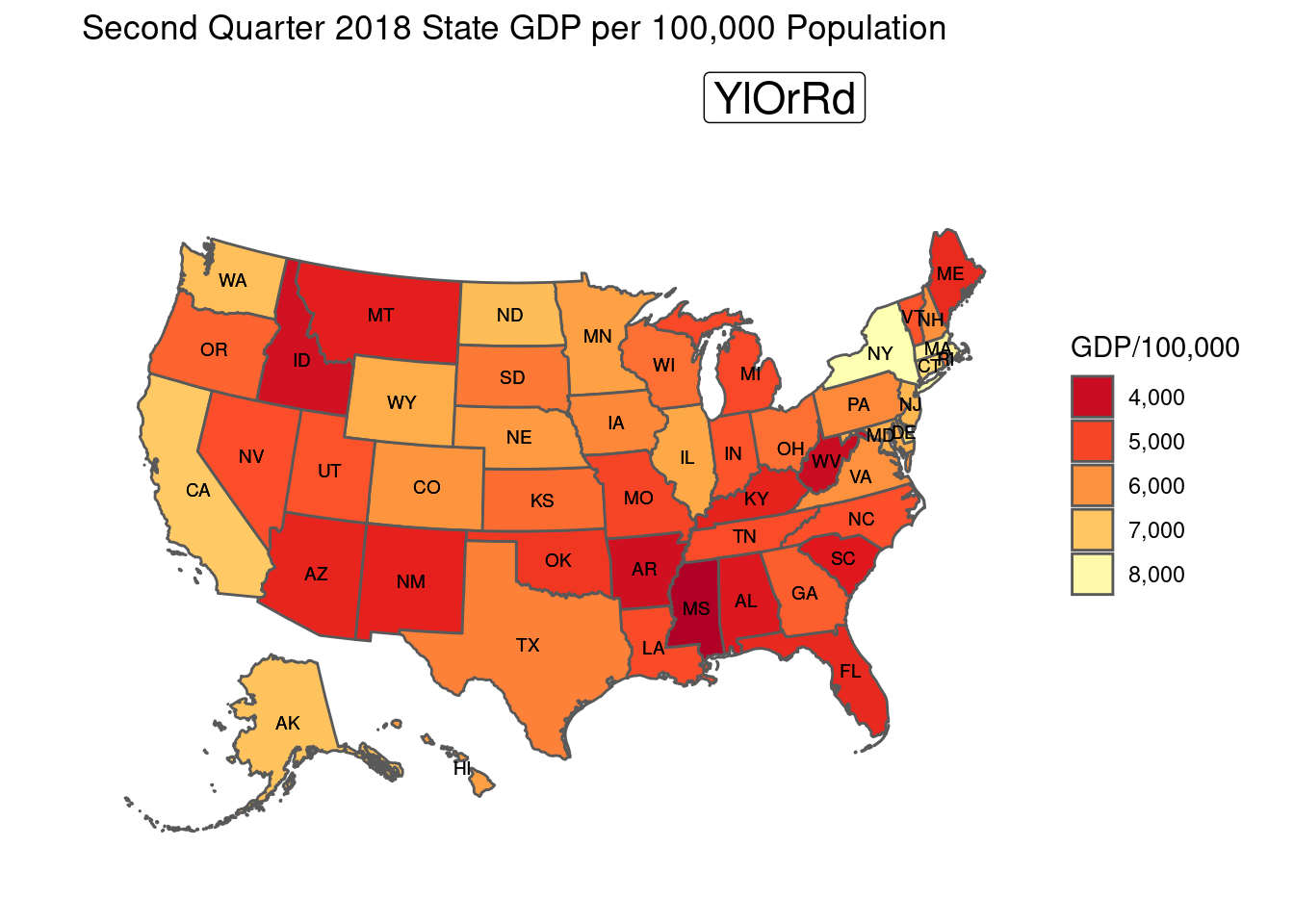
scale_fill_distiller(type = “seq”, palette = “YlOrRd”, direction = -1, labels = comma, guide = “colourbar”, aesthetics = “fill”)


Palette Snippets
Usage ggplot_map_object + [name of color scale]
Alpha_default <- scale_alpha_continuous(range = c(0.1, 1))
Alpha_75 <- scale_alpha_continuous(range = c(0.1, 0.75))
Alpha_50 <- scale_alpha_continuous(range = c(0.1, 0.50))
magma <- scale_fill_viridis_c(option="magma")
inferno <- scale_fill_viridis_c(option="inferno")
plasma <- scale_fill_viridis_c(option="plasma")
viridis <- scale_fill_viridis_c(option="viridis")
cividis <- scale_fill_viridis_c(option="cividis")
munsell_brown <- scale_fill_gradient(low = "#FBF7F6", high = "#A97263", space = "Lab", na.value = "grey50", guide = "colourbar", aesthetics = "fill")
# RColorBrewer
BluesNeg1 <- scale_fill_distiller(type = "seq", palette = "Blues", direction = -1, labels = comma, guide = "colourbar", aesthetics = "fill")
BluesPos1 <- scale_fill_distiller(type = "seq", palette = "Blues", direction = 1, labels = comma, guide = "colourbar", aesthetics = "fill")
BuGnNeg1 <- scale_fill_distiller(type = "seq", palette = "BuGn", direction = -1, labels = comma, guide = "colourbar", aesthetics = "fill")
BuGnPos1 <- scale_fill_distiller(type = "seq", palette = "BuGn", direction = 1, labels = comma, guide = "colourbar", aesthetics = "fill")
BuPuNeg1 <- scale_fill_distiller(type = "seq", palette = "BuPu", direction = -1, labels = comma, guide = "colourbar", aesthetics = "fill")
BuPuPos1 <- scale_fill_distiller(type = "seq", palette = "BuPu", direction = 1, labels = comma, guide = "colourbar", aesthetics = "fill")
GnBuNeg1 <- scale_fill_distiller(type = "seq", palette = "GnBu", direction = -1, labels = comma, guide = "colourbar", aesthetics = "fill")
GnBuPos1 <- scale_fill_distiller(type = "seq", palette = "GnBu", direction = 1, labels = comma, guide = "colourbar", aesthetics = "fill")
GreensNeg1 <- scale_fill_distiller(type = "seq", palette = "Greens", direction = -1, labels = comma, guide = "colourbar", aesthetics = "fill")
GreensPos1 <- scale_fill_distiller(type = "seq", palette = "Greens", direction = 1, labels = comma, guide = "colourbar", aesthetics = "fill")
GreysNeg1 <- scale_fill_distiller(type = "seq", palette = "Greys", direction = -1, labels = comma, guide = "colourbar", aesthetics = "fill")
GreysPos1 <- scale_fill_distiller(type = "seq", palette = "Greys", direction = 1, labels = comma, guide = "colourbar", aesthetics = "fill")
OrangesNeg1 <- scale_fill_distiller(type = "seq", palette = "Oranges", direction = -1, labels = comma, guide = "colourbar", aesthetics = "fill")
OrangesPos1 <- scale_fill_distiller(type = "seq", palette = "Oranges", direction = 1, labels = comma, guide = "colourbar", aesthetics = "fill")
OrRdNeg1 <- scale_fill_distiller(type = "seq", palette = "OrRd", direction = -1, labels = comma, guide = "colourbar", aesthetics = "fill")
OrRdPos1 <- scale_fill_distiller(type = "seq", palette = "OrRd", direction = 1, labels = comma, guide = "colourbar", aesthetics = "fill")
PuBuGnNeg1 <- scale_fill_distiller(type = "seq", palette = "PuBuGn", direction = -1, labels = comma, guide = "colourbar", aesthetics = "fill")
PuBuGnPos1 <- scale_fill_distiller(type = "seq", palette = "PuBuGn", direction = 1, labels = comma, guide = "colourbar", aesthetics = "fill")
PuBuNeg1 <- scale_fill_distiller(type = "seq", palette = "PuBu", direction = -1, labels = comma, guide = "colourbar", aesthetics = "fill")
PuBuPos1 <- scale_fill_distiller(type = "seq", palette = "PuBu", direction = 1, labels = comma, guide = "colourbar", aesthetics = "fill")
PuRdNeg1 <- scale_fill_distiller(type = "seq", palette = "PuRd", direction = -1, labels = comma, guide = "colourbar", aesthetics = "fill")
PuRdPos1 <- scale_fill_distiller(type = "seq", palette = "PuRd", direction = 1, labels = comma, guide = "colourbar", aesthetics = "fill")
PurplesNeg1 <- scale_fill_distiller(type = "seq", palette = "Purples", direction = -1, labels = comma, guide = "colourbar", aesthetics = "fill")
PurplesPos1 <- scale_fill_distiller(type = "seq", palette = "Purples", direction = 1, labels = comma, guide = "colourbar", aesthetics = "fill")
RdPuNeg1 <- scale_fill_distiller(type = "seq", palette = "RdPu", direction = -1, labels = comma, guide = "colourbar", aesthetics = "fill")
RdPuPos1 <- scale_fill_distiller(type = "seq", palette = "RdPu", direction = 1, labels = comma, guide = "colourbar", aesthetics = "fill")
RedsNeg1 <- scale_fill_distiller(type = "seq", palette = "Reds", direction = -1, labels = comma, guide = "colourbar", aesthetics = "fill")
RedsPos1 <- scale_fill_distiller(type = "seq", palette = "Reds", direction = 1, labels = comma, guide = "colourbar", aesthetics = "fill")
YlGnBuNeg1 <- scale_fill_distiller(type = "seq", palette = "YlGnBu", direction = -1, labels = comma, guide = "colourbar", aesthetics = "fill")
YlGnBuPos1 <- scale_fill_distiller(type = "seq", palette = "YlGnBu", direction = 1, labels = comma, guide = "colourbar", aesthetics = "fill")
YlGnNeg1 <- scale_fill_distiller(type = "seq", palette = "YlGn", direction = -1, labels = comma, guide = "colourbar", aesthetics = "fill")
YlGnPos1 <- scale_fill_distiller(type = "seq", palette = "YlGn", direction = 1, labels = comma, guide = "colourbar", aesthetics = "fill")
YlOrBrNeg1 <- scale_fill_distiller(type = "seq", palette = "YlOrBr", direction = -1, labels = comma, guide = "colourbar", aesthetics = "fill")
YlOrBrPos1 <- scale_fill_distiller(type = "seq", palette = "YlOrBr", direction = 1, labels = comma, guide = "colourbar", aesthetics = "fill")
YlOrRdNeg1 <- scale_fill_distiller(type = "seq", palette = "YlOrRd", direction = -1, labels = comma, guide = "colourbar", aesthetics = "fill")
YlOrRdPos1 <- scale_fill_distiller(type = "seq", palette = "YlOrRd", direction = 1, labels = comma, guide = "colourbar", aesthetics = "fill")
BrBGNeg1 <- scale_fill_distiller(type = "seq", palette = "BrBG", direction = -1, labels = comma, guide = "colourbar", aesthetics = "fill")
BrBGPos1 <- scale_fill_distiller(type = "seq", palette = "BrBG", direction = 1, labels = comma, guide = "colourbar", aesthetics = "fill")
PiYGNeg1 <- scale_fill_distiller(type = "seq", palette = "PiYG", direction = -1, labels = comma, guide = "colourbar", aesthetics = "fill")
PiYGPos1 <- scale_fill_distiller(type = "seq", palette = "PiYG", direction = 1, labels = comma, guide = "colourbar", aesthetics = "fill")
PRGnNeg1 <- scale_fill_distiller(type = "seq", palette = "PRGn", direction = -1, labels = comma, guide = "colourbar", aesthetics = "fill")
PRGnPos1 <- scale_fill_distiller(type = "seq", palette = "PRGn", direction = 1, labels = comma, guide = "colourbar", aesthetics = "fill")
PuOrNeg1 <- scale_fill_distiller(type = "seq", palette = "PuOr", direction = -1, labels = comma, guide = "colourbar", aesthetics = "fill")
PuOrPos1 <- scale_fill_distiller(type = "seq", palette = "PuOr", direction = 1, labels = comma, guide = "colourbar", aesthetics = "fill")
RdBuNeg1 <- scale_fill_distiller(type = "seq", palette = "RdBu", direction = -1, labels = comma, guide = "colourbar", aesthetics = "fill")
RdBuPos1 <- scale_fill_distiller(type = "seq", palette = "RdBu", direction = 1, labels = comma, guide = "colourbar", aesthetics = "fill")
RdGyNeg1 <- scale_fill_distiller(type = "seq", palette = "RdGy", direction = -1, labels = comma, guide = "colourbar", aesthetics = "fill")
RdGyPos1 <- scale_fill_distiller(type = "seq", palette = "RdGy", direction = 1, labels = comma, guide = "colourbar", aesthetics = "fill")
RdYlBuNeg1 <- scale_fill_distiller(type = "seq", palette = "RdYlBu", direction = -1, labels = comma, guide = "colourbar", aesthetics = "fill")
RdYlBuPos1 <- scale_fill_distiller(type = "seq", palette = "RdYlBu", direction = 1, labels = comma, guide = "colourbar", aesthetics = "fill")
RdYlGnNeg1 <- scale_fill_distiller(type = "seq", palette = "RdYlGn", direction = -1, labels = comma, guide = "colourbar", aesthetics = "fill")
RdYlGnPos1 <- scale_fill_distiller(type = "seq", palette = "RdYlGn", direction = 1, labels = comma, guide = "colourbar", aesthetics = "fill")
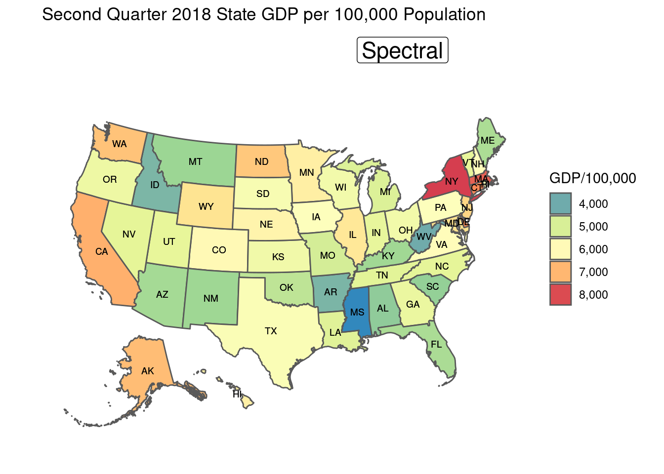
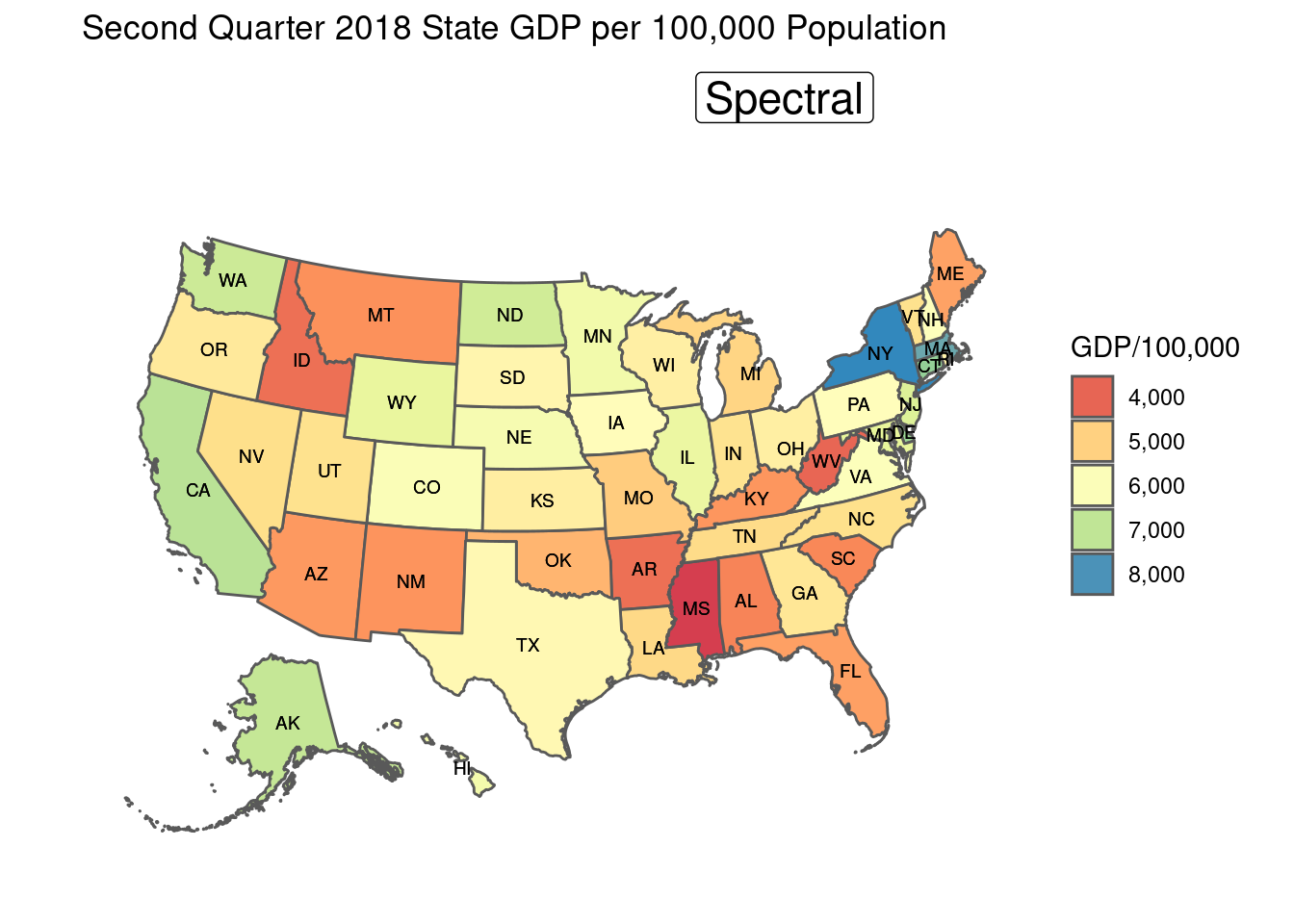
SpectralNeg1 <- scale_fill_distiller(type = "seq", palette = "Spectral", direction = -1, labels = comma, guide = "colourbar", aesthetics = "fill")
SpectralPos1 <- scale_fill_distiller(type = "seq", palette = "Spectral", direction = 1, labels = comma, guide = "colourbar", aesthetics = "fill")
AccentNeg1 <- scale_fill_distiller(type = "seq", palette = "Accent", direction = -1, labels = comma, guide = "colourbar", aesthetics = "fill")
AccentPos1 <- scale_fill_distiller(type = "seq", palette = "Accent", direction = 1, labels = comma, guide = "colourbar", aesthetics = "fill")
Dark2Neg1 <- scale_fill_distiller(type = "seq", palette = "Dark2", direction = -1, labels = comma, guide = "colourbar", aesthetics = "fill")
Dark2Pos1 <- scale_fill_distiller(type = "seq", palette = "Dark2", direction = 1, labels = comma, guide = "colourbar", aesthetics = "fill")
PairedNeg1 <- scale_fill_distiller(type = "seq", palette = "Paired", direction = -1, labels = comma, guide = "colourbar", aesthetics = "fill")
PairedPos1 <- scale_fill_distiller(type = "seq", palette = "Paired", direction = 1, labels = comma, guide = "colourbar", aesthetics = "fill")
Pastel1Neg1 <- scale_fill_distiller(type = "seq", palette = "Pastel1", direction = -1, labels = comma, guide = "colourbar", aesthetics = "fill")
Pastel1Pos1 <- scale_fill_distiller(type = "seq", palette = "Pastel1", direction = 1, labels = comma, guide = "colourbar", aesthetics = "fill")
Pastel2Neg1 <- scale_fill_distiller(type = "seq", palette = "Pastel2", direction = -1, labels = comma, guide = "colourbar", aesthetics = "fill")
Pastel2Pos1 <- scale_fill_distiller(type = "seq", palette = "Pastel2", direction = 1, labels = comma, guide = "colourbar", aesthetics = "fill")
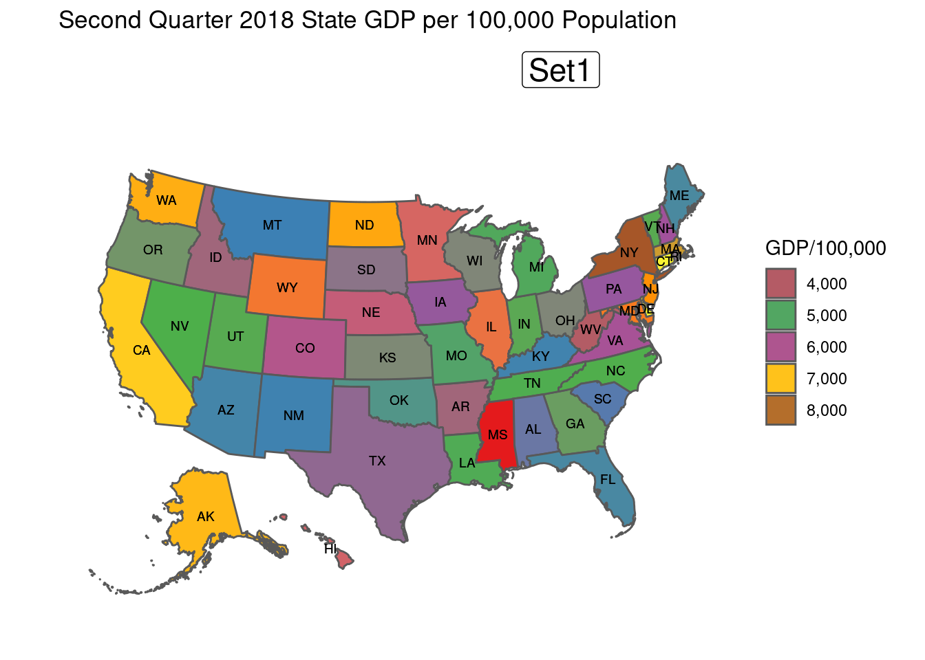
Set1Neg1 <- scale_fill_distiller(type = "seq", palette = "Set1", direction = -1, labels = comma, guide = "colourbar", aesthetics = "fill")
Set1Pos1 <- scale_fill_distiller(type = "seq", palette = "Set1", direction = 1, labels = comma, guide = "colourbar", aesthetics = "fill")
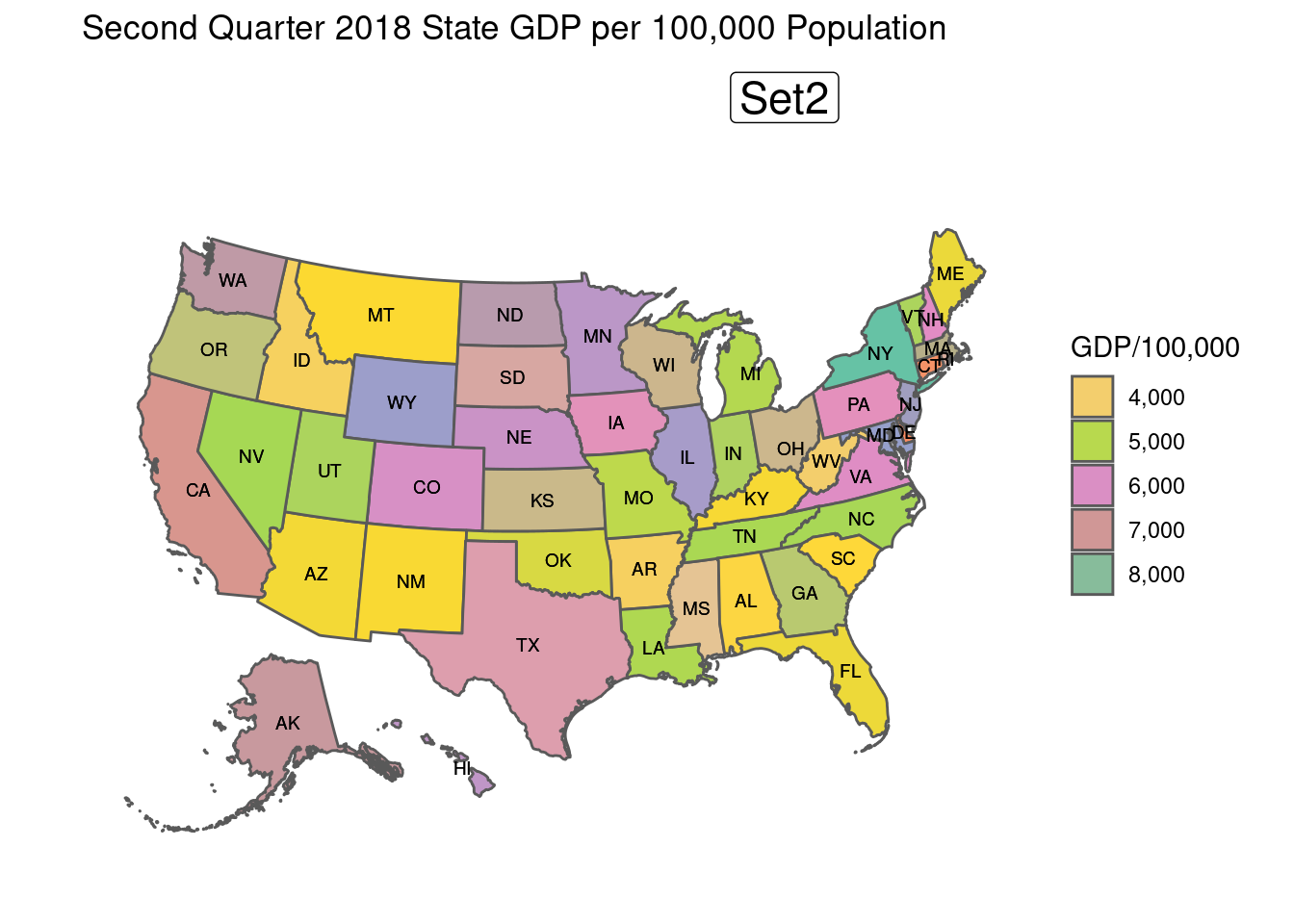
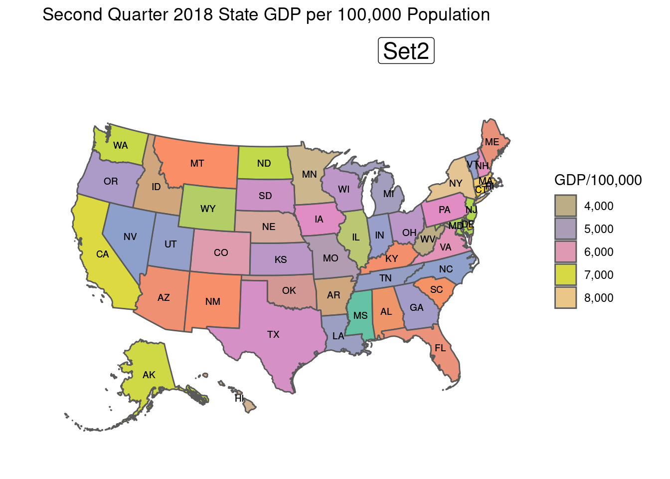
Set2Neg1 <- scale_fill_distiller(type = "seq", palette = "Set2", direction = -1, labels = comma, guide = "colourbar", aesthetics = "fill")
Set2Pos1 <- scale_fill_distiller(type = "seq", palette = "Set2", direction = 1, labels = comma, guide = "colourbar", aesthetics = "fill")
Set3Neg1 <- scale_fill_distiller(type = "seq", palette = "Set3", direction = -1, labels = comma, guide = "colourbar", aesthetics = "fill")
Set3Pos1 <- scale_fill_distiller(type = "seq", palette = "Set3", direction = 1, labels = comma, guide = "colourbar", aesthetics = "fill")
Credits
- R Development Core Team (2008). R: A language and environment for statistical computing. R Foundation for Statistical Computing, Vienna, Austria. ISBN 3-900051-07-0, URL http://www.R-project.org.
- Simon Urbanek and Jeffrey Horner (2015). Cairo: R graphics device using cairo graphics library for creating high-quality bitmap (PNG, JPEG, TIFF), vector (PDF, SVG, PostScript) and display (X11 and Win32) output. R package version 1.5-9. https://CRAN.R-project.org/package=Cairo
- H. Wickham. ggplot2: Elegant Graphics for Data Analysis. Springer-Verlag New York, 2016
- Hao Zhu (2018). kableExtra: Construct Complex Table with ‘kable’ and Pipe Syntax. R package version 0.9.0. https://CRAN.R-project.org/package=kableExtra
- Yihui Xie (2018). knitr: A General-Purpose Package for Dynamic Report Generation in R. R package version 1.20. Yihui Xie (2015) Dynamic Documents with R and knitr. 2nd edition. Chapman and Hall/CRC. ISBN 978-1498716963 Yihui Xie (2014) knitr: A Comprehensive Tool for Reproducible Research in R. In Victoria 6. Stodden, Friedrich Leisch and Roger D. Peng, editors, Implementing Reproducible Computational Research. Chapman and Hall/CRC. ISBN 978-1466561595
- Charlotte Wickham (2018). munsell: Utilities for Using Munsell Colours. R package version 0.5.0. https://CRAN.R-project.org/package=munsell
- Erich Neuwirth (2014). RColorBrewer: ColorBrewer Palettes. R package version 1.1-2. https://CRAN.R-project.org/package=RColorBrewer
- Hadley Wickham (2018). scales: Scale Functions for Visualization. R package version 1.0.0.https://CRAN.R-project.org/package=scales
- Pebesma, E., 2018. Simple Features for R: Standardized Support for Spatial Vector Data. The R Journal, https://journal.r-project.org/archive/2018/RJ-2018-009/
- Kyle Walker (2018). tidycensus: Load US Census Boundary and Attribute Data as ‘tidyverse’ and22 ‘sf’-Ready Data Frames. R package version 0.8.1. https://CRAN.R-project.org/package=tidycensus
- Hadley Wickham (2017). tidyverse: Easily Install and Load the ‘Tidyverse’. R package version 1.2.1. https://CRAN.R-project.org/package=tidyverse
“Source: Bureau of Economic Analysis, Gross Domestic Product By State, 2nd Quarter 2018 https://goo.gl/Jc6XyK”↩︎